Zero-shot Object Localization With Image-Text Models and Saliency Methods
Recent works in computer vision have proposed image-text foundation models that subsume both vision and language pre-training. Methods such as CLIP, ALIGN, and COCA demonstrated success in generating powerful representations for a variety of downstream tasks, from traditional vision tasks such as image classification to multimodal tasks such as visual question answering and image captioning. In particular, these methods showed impressive zero-shot capabilities. CLIP and COCA was able to achieve 76.2% and 86.3% top-1 classification accuracy on Imagenet, respectively, without explicitly training on any images from the dataset. Motivated by these observations, in this work, we explore the effectiveness of image-text foundation model representations in zero-shot object localization. We propose a variant of Score-CAM that considers both Vision and Language inputs (VL-Score). VL-Score generates a saliency map for an image conditioning on a user-provided textual query, from intermediate features of pre-trained image-text foundation models. When the query asks for an object in the image, our method would return the corresponding localization result. We quantitively evaluate our method on the ImageNet validation set, and demonstrate comparative ground truth localization accuracy with state of the art of weakly supervised object localization methods. We also provide a streamLit interface that enable users to experiment with different image and text combinations. The code is released on Github.
- Introduction and Motivation
- Related Literature
- Methodology
- Data and Evaluation Plan
- Experiment Results and Analysis
- Future Work
- StreamLit Interface
- Conclusion
- Reference
Introduction and Motivation
Deep neural networks have achieved notable success in the field of object recognition. However, the most accurate models require large number of annotations. For the object localization task that seeks to find the area of the object of interest in an given image, fully supervise methods need instance level labels such as bounding boxes and pivot points, which are highly costly. This leads to the emergence of weakly supervised object localization. With only image-level supervision, it can still achieve good localization accuracy. While traditional weakly supervised localization methods provide an alternative that saves annotation time, in the test time, they are limited to predict on the predetermined object classes observed during training. Therefore, to locate novel object categories, the model has to be finetuned on a new dataset. Zero-shot methods[7, 8] aim to address this issue and achieve comparative localization results for out of distribution labels without additional training. In this work, we propose a framework that combines pre-trained image-text models from web data without human annotation, and saliency methods, for the zero-shot object localization task.
Recent works in computer vision have proposed image-text foundation models that subsume both vision and language pre-training. Methods such as CLIP [2], ALIGN [13], and COCA [12] demonstrated success in generating powerful representations for a variety of downstream tasks, from traditional vision tasks such as image classification to multimodal tasks such as visual question answering and image captioning. In particular, these methods showed impressive zero-shot capabilities. CLIP and COCA was able to achieve 76.2\% and 86.3\% top-1 classification accuracy on Imagenet, respectively, without explicitly training on any images from the dataset. Motivated by these observations, in this work, we explore the effectiveness of image-text foundation model representations in zero-shot object localization. We propose a variant of Score-CAM[3] that considers both Vision and Language inputs (VL-Score). VL-Score generates a saliency map for an image conditioning on a user-provided textual query, from intermediate features of pre-trained image-text foundation models. When the query asks for an object in the image, our method would return the corresponding localization result. We quantitively evaluate our method on the ImageNet validation set, and demonstrate comparative ground truth localization accuracy with state of the art of weakly supervised object localization methods. While our framework may be applied to image-text models in general, in this report we build our implementation on top of CLIP, since we do not have access to other pre-trained models at the time of this work. We examine internal features of both the CNN and ViT architecture for CLIP’s image encoders, and evaluate the influence of different features on our localization objective, both qualitatively and quantitively. We also provide an streamLit interface that enable to users to experiment with different image and text combinations. The code is released on Github.
Related Literature
Image-Text Foundation Models
A recent line of research in computer vision focuses on pre-training with image and text jointly to learn multimodal representations. One paradigm of works [2][13],demonstrated success by training two encoders simultaneuously with contrastive loss. The dual-encoder model consists of an image and text encoder and embed images and texts in the same latent space. These models are typically trained with noisy webly data that are image and text pairs. Another line of work follows an encoder-decoder architecture. During pre-training, the encoder takes images as input, and the decoder is applied with a language modeling loss. As a further step, the most recent work [12] combines both architectures and achieves the state of art results on a variety of vision and language tasks.
In this work, we utilize CLIP (Radford, et al. 2021), an image-text foundation model with a dual-encoder architecture. The encoders are trained in parallel with web collected images and corresponding captions. During training, CLIP aligns the outputs from the image and text encoder in the same latent space.
The detailed structure is shown in Fig.1. For each training step, a batch of n image and text pairs is sampled. The matching pairs are treated as positive examples, and unmatching are negative examples. Then the model computes the inner product of embeddings from the encoders for each pair and applies a contrastive loss.
In the test time, given a set of possible labels and an input image, CLIP places each label within a prompt that can be in the form of “an image of a [label].” and uses the pretrained text encoder to embed the prompts. Then it computes the inner product between the text embeddings and the image embedding from the image encoder. Finally, the label whose prompt generates the highest similarity score will be the prediction answer.
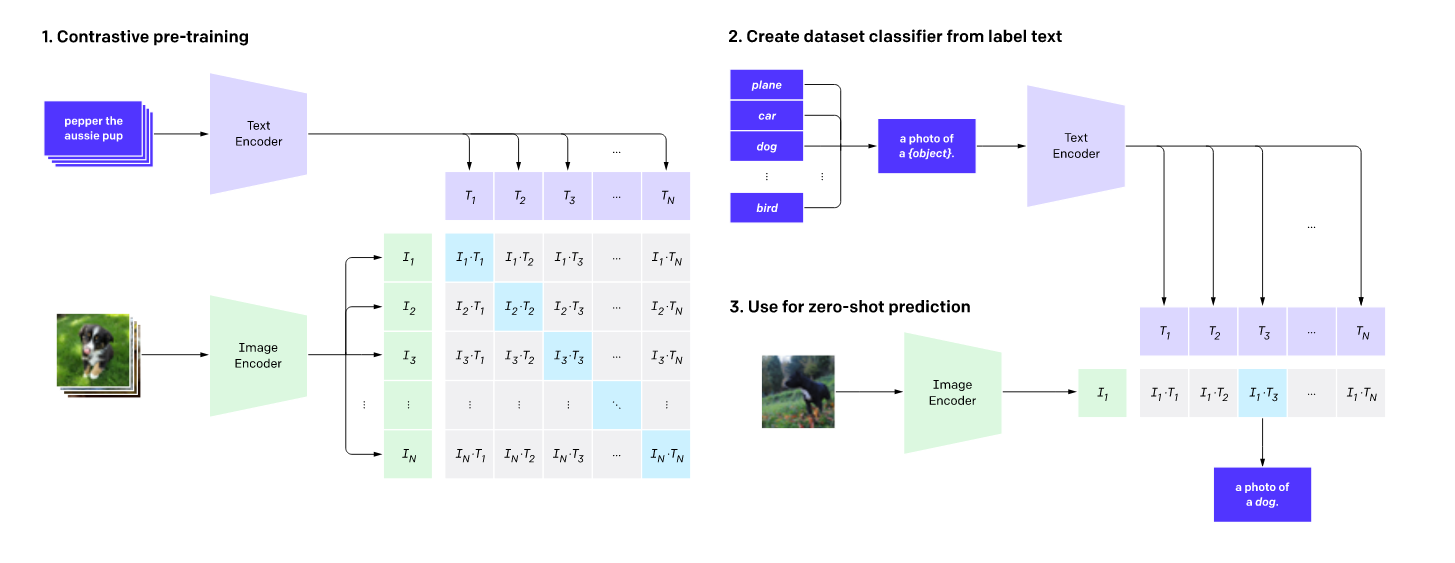
Fig 1. CLIP’s structure. From CLIP (Radford, et al. 2021)
Saliency Methods
Saliency methods such as CAM [4] and Grad-CAM [5] have shown to generate class dependent heapmaps that highlight areas containing objects of the given class in an input image from intermediate outputs of pre-trained image classification models, such as VGG and ResNet. The generated saliency maps can be directly used to perform localization tasks by drawing bounding boxes around the most highlighted region.
Score-CAM (Wang, et al. 2020) is a another method to generate saliency maps for CNN based image classifiers. It often produces more accurate and stable results than gradient based methods from experimental results. According to Fig. 2, given an input image, score cam takes the activation maps from the last convolution layer, and uses these maps as masks over the the input image. The masked input images are processed by the CNN again to generate a weight for each activation map. The weights are normalized the weighted sum of the maps is used as the final output.
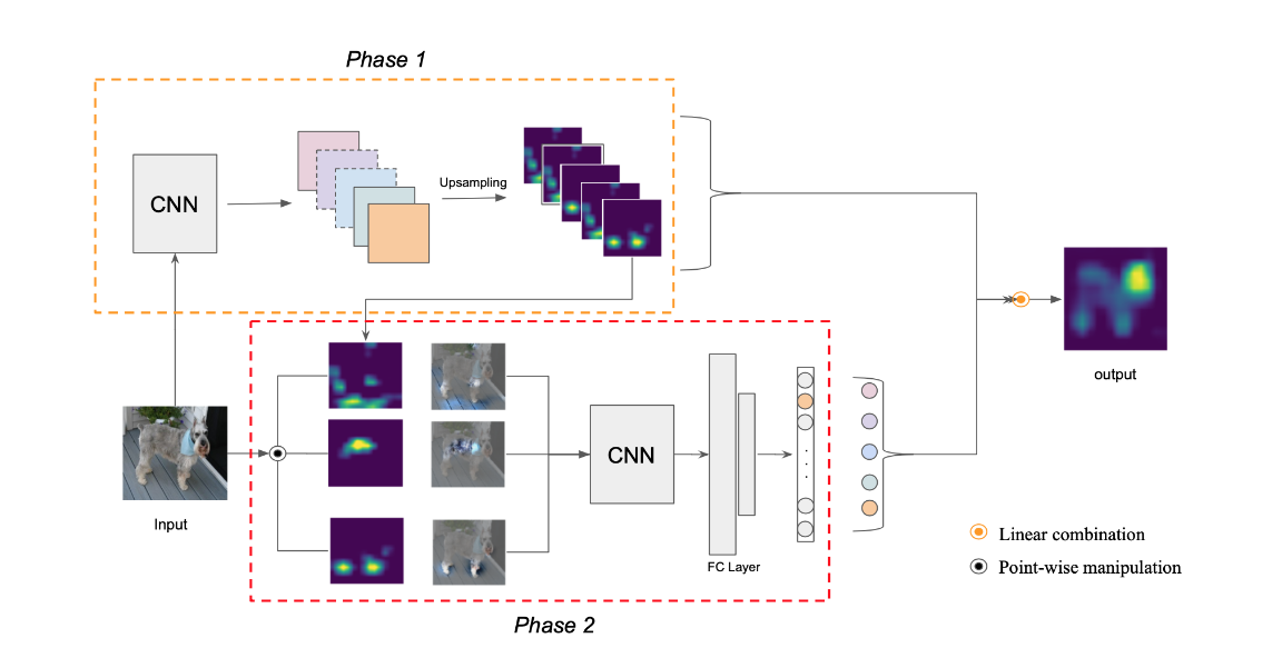
Fig 2. Score CAM’s structure. From Score-CAM (Wang, et al. 2020)
More detaily, given an input image and a CNN based image processor f, ScoreCAM will use feature maps from convolutional layer of f as a mask and applied the mask over the input. With regard to the masked image, ScoreCAM uses the image processor to process the masked image and use the logit for class c as the feature map’s contribution score to c. In the end, the weighted sum of the feature maps are calculated using the contribution scores. The result will be a saliency map for class c.
Comparing to saliency methods that utilizes gradients, Score-CAM often results in more stable saliency maps. Additionally, it adapts to CLIP naturally, by changing the definition of the score from the logit of the target class to the inner product between the masked input image embedding resulted from the CLIP image encoder and the text embedding generated by the text encoder.
Vision Transformers (ViT)
Vision Transformers are competitive alternative to convolutional neural networks to perform vision processing tasks. The architecture of ViT is mostly the same as standard Transformers, which model the relationships between pairs of input tokens in sequence. The difference mainly lies in the definition of tokens. For standard Transformers each token can be a word in a sentence, where in ViT, a token is a patch of the original image. Input images to ViT are split into fixed-size patches and rearranged into a sequence. Then added with position embeddings, the corresponding vectors will be sent to a standard transformer encoder.
As shown in Fig 3, inside transformer block l, token embedding in layer l-1 will be first linear projected to query, key, values. Then the multihead-attention module will compute inter token attention, and finally generate layer l’s embedding. In this project, we experimented with all the intermediate outputs mentioned above.
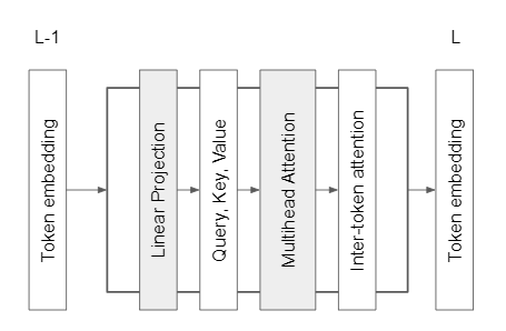
Fig 3. ViT’s structure.
Methodology
Combine Image-Text Models and Saliency Methods
To generate text dependent saliency maps from intermediate features of an image-text model, we propose VL-Score, a variant of Score-CAM that accounts for both vision and language inputs. Given an image and a class label embedding in a prompt, we first apply the image and text encoder to embed the image and text inputs into the same latent space. After this forward pass, we extract intermdiate features from a specific layer of the image encoder. For instance, if the image encoder builds upon a CNN architecture, we can extract the activations after the a specific convolutional layer l. The extracted features will be normalized to the scale between 0 and 1 and reshaped into masks that have the shape of the input image. After applying the feature masks to the original input, the masked images will be sent to image encoder to compute the masked image embeddings. These embeddings are then dot producted with the prompt’s embedding to compute the similar of each feature map to the given sentence. The similarity score are then normalized and used to compute the final saliency map with the feature maps, as shown in Figure 4.
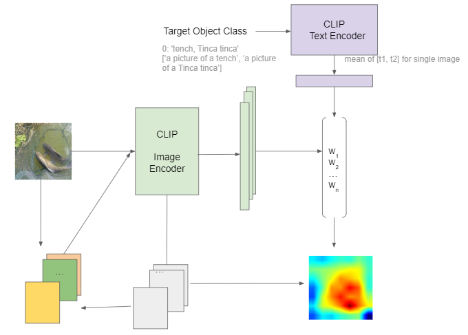
Fig 4. Our method pipeline.
Similar to Score-CAM, our method uses a base image, which is by default an image whose pixel values are all zero, and computes the dot product of the base image’s embedding and the prompt’s embedding as the base score. However, we do not substract this base score from the scores of each feature map. Instead, we use the base score as cap such that we only keep the feature maps whose scores are higher than the base. If none of the feature map has a higher score, our method determines that the object of interest is not present in the given image. The scores that are higher than the base are put into a softmax with a temperature. The results are used to compute the weight sum of corresponding feature maps as the final output.
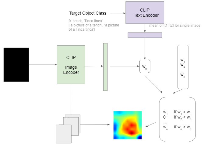
Fig 5. Our method pipeline’s base image.
Image Encoder CNN
In this project, we use CLIP as the image-text model since it has released pre-trained versions. In particular, it has two types of pretrained image encoders, based on CNN and ViT architectures. For CNN based encoders, it releases models including ResNet 50[9], Resnet 101, Resnet 50 * 4, etc. The definition of feature maps in the CNN architecture is natural. Typically, the features are extracted from last convolutional layer of the encoder. The detailed algorithm of VL-Score for CNN base architecture is shown in Figure 6.
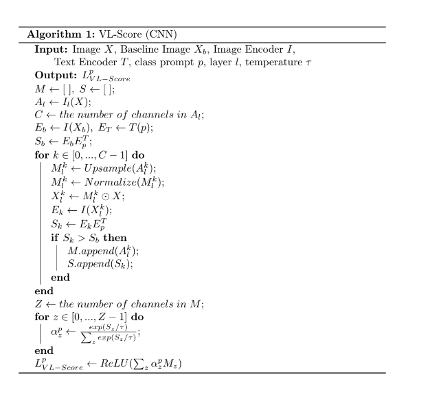
Fig 6. Algorithm of VL-score for CNN based architecture.
Image Encoder ViT
On the other hand, the definition of feature maps in ViT base encoders is not as obvious. Here, we explore several methods of extracting intermediate features. One way of feature extraction analagous to the case in CNN encoders is to directly use the output of a transformer block. The patches embeddings of shape n x d, where n is equal to w x h, can be reshaped into w x h x d. Then we can treat each slice of the embeddings in the last dimension as a feature. Another common way is to utilize the attention outputs from an transformer block. For a block that has T heads, there are T x n attention scores between the class token to each of the n patch tokens. Then these attentions can be reshaped into T x w x h and sliced along the last dimension. Besides directly using a transformer block’s output, [11] has shown that the intermediate outputs such as keys, queries, and values inside a transformer block can preserve structural information for ViT in DINO. Therefore, we also experimented with using these intermediate features and applied PCA in attempt to obtain more structured feature maps.
Fig 7 illustrates the feature maps acquired by each of the four methods. We observe that for CLIP ViT-base/16, the inter-token attention, token embedding and query, key, value(QKV) maps highlight sparsely connected regions. After applying PCA, the most principle components of query embeddings show more structured regions such as a human’s head or a fish. However, within a single feature, multiple semantic regions can be highlighted simultaneuously.

Fig 7. ViT four methods are experimented to check the feature map performance.
Data and Evaluation Plan
We quantitively evaluate our zero-shot localization approach on the ImageNet 2012 validation dataset. The dataset consists of 50000 images and 1000 classes. Each image has a single class label for the main objects. Each class label may have multiple synonyms. Additionally, an image may contain multiple ground truth localization bounding boxes.
There are 4 evaluation metrics: box IOU, groud truth localization accuracy, top-1 localization accuracy, and top-5 localization accuracy. Given an input label, our method may predict from zero to multiple bounding boxes. \(box\_iou = \frac{\text{area of intersection}}{\text{area of union}}\). For images that contain several ground truth bounding boxes, we calculate box_iou with regard to every pair of predicted target and ground truth target, and pick the largest one to be the box_iou result. \(box\_iou_{final} = max([box\_iou(gt_{i}, predict_{j}) i \in m, j \in n])\). If the box_iou of an image is larger than 0.5, the predict is considered as correct for ground truth localization accuracy. For top 1 localization accuracy, box_iou needs to be larger than 0.5 and the predicted top 1 label should be the correct label. Top 5 localization accuracy means the box_iou needs to be larger than 0.5 and correct label should fall into top 5 predicted labels.
When construting the textual prompt as the input to the text encoder given a label, we use the template “an image of a {label}.” to create the sentence. In the case where there are multiple synonyms for the given label, we embed each synonym into the template, and use the average of the embedding outputs from the text encoder. We note that prompt engineering is a seperate research domain, and the offical Github repository of the CLIP project provides a set of templates for the ImageNet dataset.
Experiment Results and Analysis
We first present our quantitive results on the ImageNet validation set with Resnet50 backbone. As shown in Table 1, our pipeline reach 66.60% for ground truth localization accuracy. Considering VL-Score is a zero shot localization method, it still achieves comparative ground truth accuracy to state of the art weakly supervised object localization methods, and outperforms some of them. High ground truth accuracy suggests that 1) the features maps in the last layer of CLIP’s CNN image encoder captures the structure the main objects in an image; and 2) the cosine similarity between the feature masked image’s embedding and the label’s embedding serves as a good proxy for measuring the contribution of the feature map to the prediction of that label.
On the other hand, the top-1 and top-5 localization accuracy are significantly lower. While the top-5 accuracy still outperforms the vanilla CAM method, the top-1 accuracy is lower than CAM. This is due to the fact the zero-shot classification accuracy of the Resnet50 model on ImageNet is significantly than the WSOL models directly trained on ImageNet. The issue may be alleviated by using more accurate pre-trained image encoders from CLIP, such as Resnet101, Resnet50x4, and Resnet50x16. Due to limited computational resources, we only evaluated the Resnet101 architecture, which shows better top-1 and top-5 localization accuracy than Resnet50 in some settings, as shown in Table 2. Another common approach in localization models is to use two prediction heads: one for bounding box prediction, and the other for classification prediction. We may utilize Resnet50 for fast bounding box prediction and another pre-trained backend from CLIP for classificaion results. It is noteworthy that despite Resnet50’s low classification accuracy, the intermediate features are able to capture the shape of objects from novel categories.
| Method | Backbone | GT-known Loc | Top-5 Loc | Top-1 Loc |
|---|---|---|---|---|
| ResNet50-CAM[14] | ResNet50 | 51.86 | 49.47 | 38.99 |
| ADL[15] | ResNet50 | 61.04 | - | 48.23 |
| FAM[19] | ResNet50 | 64.56 | - | 54.46 |
| PSOL[16] | ResNet50 | 65.44 | 63.08 | 53.98 |
| I^2C[17] | ResNet50 | 68.50 | 64.60 | 54.83 |
| SPOL[18] | ResNet50 | 69.02 | 67.15 | 59.14 |
| BGC [20] | ResNet50 | 69.89 | 65.75 | 53.76 |
| VL-Score (Ours) | ResNet50 | 66.93 | 57.20(cls 85.26) | 39.50(cls 58.64) |
Table 1: Comparision with other classical work. Our pipeline’s best performance can reach 66.60% ground truth localization.
Specific case analysis is shown in Fig. 8 and Fig. 9. In these cases, we examine VL-Score’s localization ability by feeding the ground truth ImageNet label to the model. For successful cases in Fig. 8, we can see the most activated area focuses on the interested object and captures features, such as head and body pretty well. However, there are also cases focusing on the non-ideal features. For instance in Fig 9’s second column, the most activated area is somewhere on the wall. But the interested object is the dog.
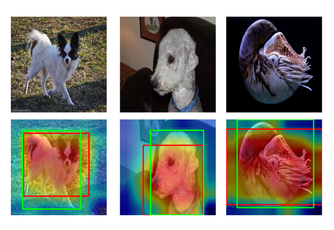
Fig 8. Good performance experiment result.
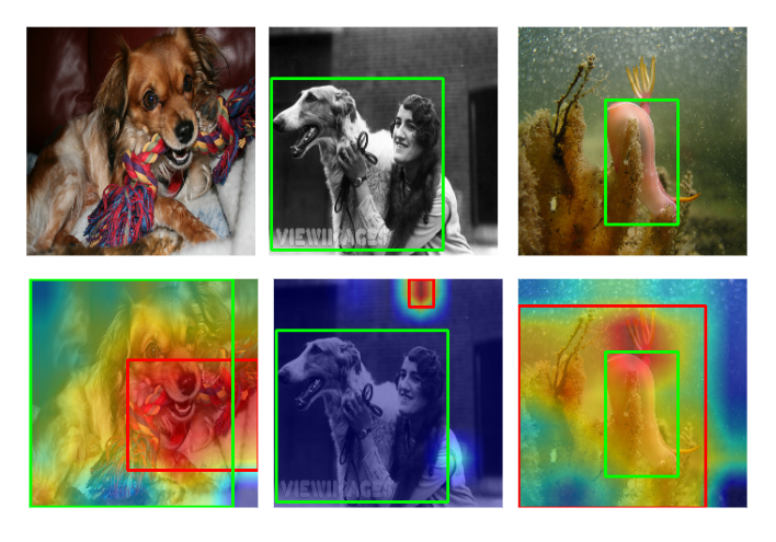
Fig 9. Non-ideal performance experiment result.
In addtion to CNN-based architectures, we test VL-Score on ViT-based image encoders from CLIP. Table 2 shows detailed experiment result using different backbone and CAM threshold. While the performaces of Resnet50 and Resnet101 are comparable, the results from ViT are significantly lower. The main reason that accounts for this phenomenon is the features map we extracted fails to identify the substructures of the interested object. Each feature map often highlights large connected regions that include multiple objects of interest, or scattered small regions. This leads to two issues: 1) each feature map does not capture the semantic structure of a single object, and therefore cannot reflect the contribution of this feature map in predicting the object of interest accurately; 2) when the feature maps are aggregated, scattered small regions that does not belong to the interested object class are also highlighted, since they often cooccur with the object of interest.
| Method | CAM threshold | box_iou | GT-known Loc | Top-1 Loc | Top-5 Loc |
|---|---|---|---|---|---|
| ResNet50 | 0.55 | 0.56 | 64.24% | 37.65% | 54.90% |
| 0.60 | 0.57 | 66.93% | 39.30% | 57.20% | |
| 0.65 | 0.57 | 66.60% | 39.20% | 57.08% | |
| ResNet101 | 0.55 | 0.55 | 64.44% | 38.94% | 55.50% |
| 0.60 | 0.55 | 65.40% | 39.5% | 56.31% | |
| 0.65 | 0.54 | 63.49% | 38.39% | 54.71% | |
| VIT(ImageNet first 10k images) | 0.55 | 0.30 | 20.80% | 14.63% | 19.57% |
| 0.60 | 0.25 | 15.08% | 10.85% | 14.18% | |
| 0.65 | 0.19 | 9.66% | 6.82% | 9.1% |
Table 2: Overall experiment result.
We illustrate this phenomenon by comparing the generated saliency map for an example image where a man is holding a fish, with both the CNN-based image encoder (Fig 11.), and the ViT-based encoder (Fig 12.) from CLIP. For each setting, there are four textual signals, ‘a picture of a man.’, ‘a picture of a face.’, ‘a picture of a man’s face.’, and ‘a picture of a fish.’. Different text signals generate different contribution scores for each feature map, and the resulting saliency map changes accordingly. While the saliency map does not alway highlight the intended regions in Fig 12., only a few contiguous regions are highlighted. On the contrary, in addition to potential objects of interest, many scattered small regions are highlighted in the background. Across different text signal inputs, some regions are consistently highlighted, such as the hat, since it co-occurs with other object regions in the original feature maps.
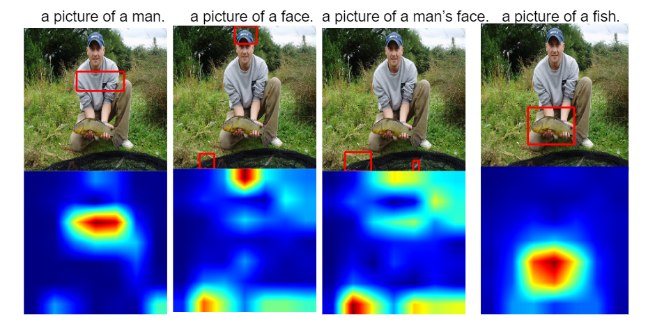
Fig 11. Case study given different label input, with backbone ResNet101.
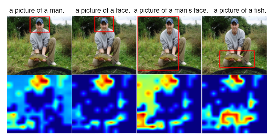
Fig 12. Case study given different label input, with backbone ViT.
In Fig 13 and 14, we can see the threshold for filtering out background pixels also has influence over the localization accuracy. Heatmap has different intensity in pixel representing the activation level of the area. Pixels with higher intensity are regarded as more activated feature area. When the threshold is higher, more pixels will be filtered and therefore the bounding boxes will be smaller and more likely to be seperated into multiple boxes. When there are multiple ground truth instances, such as multiple hens in the example image, higher threashold can help slice the most activated areas in heatmap. However, threshold is not the higher, the better. In the upper histogram in Fig 13, for both ResNet 50 and ResNet 101, we can see when threshold = 0.6, the accuracy with known ground truth is highest compared with case threshold 0.55 and 0.65. Thus, threshold can be a hyperparameter affecting the localization accuracy.
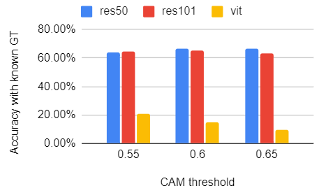
Fig 13. Box iou’s relationship with CAM threshold.
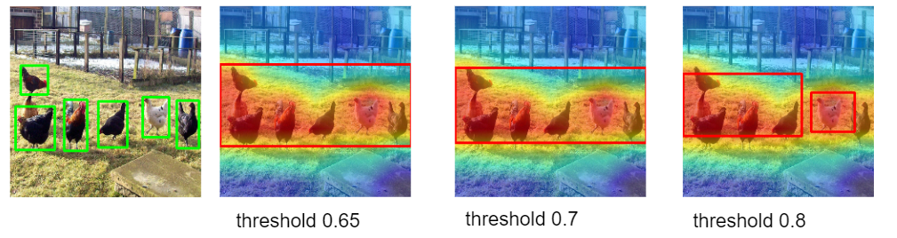
Fig 14. Bounding box changes as threshold changes.
Future Work
The goal of this work is to demonstrate the zero-shot capability of image-text models in the localization task with saliency methods. In this writing, we focused on CLIP as it was the only publicly accessible pretrained model. The natural question to ask is whether our proposed method would result in similar performance on other image text models. Additionally, we only tested several available architectures of CLIP due to computation limit, and results from other architectures may reveal new insights into our problem. Although we explored various approaches of extracting useful feature maps from the ViT image encoder, our method did not show compelling results. This issue may be further explored in the future.
StreamLit Interface
To make our work more interactive, we provide a StreamLit Interface for users to upload their own image and experiment with different text descriptions to the localization and saliency results. Note that running with CPU can be extremely slow. Detailed instructions on how to setup this interface is provided in https://github.com/mxuan0/zeroshot-localization.git.
Figure 15 shows an illustration of how to use the interface. The user can select their intended model, layer, and bounding box thresholds. After uploading an image and enter a text description, the program can be run by clicking ‘Find it!’.

Fig 15. StreamLit Interface.
Conclusion
In this work, we propose a variant of Score-CAM that seeks to utilize internal features of image-text models for the zero-shot object localization task. We evaluate our method on CLIP with multiple architectures of the image encoder. We show that VL-Score can perform zero-shot object localization with comparable ground truth localization accuracy to state of the art to WSOL methods on the ImageNet validation set. At the same time, our method has the following limitations. When there are m multiple ground truth bounding boxes, the pipeline is far from predict exactly m bounding boxes. In most cases it only predicts one whole box or two boxes. Additionally, finding suitable activation maps from ViT image encoder remains a problem. Directly extracting features from intermediate layers does not yield intended performance.
Reference
[1] Dosovitskiy, Alexey, et al. “An image is worth 16x16 words: Transformers for image recognition at scale.” arXiv preprint arXiv:2010.11929 (2020).
[2] Radford, Kimm et al. “Learning Transferable Visual Models From Natural Language Supervision.” Arxiv. 2021.
[3] Wang et al. “Score-CAM: Score-Weighted Visual Explanations for Convolutional Neural Networks.” Conference on Computer Vision and Pattern Recognition. 2019.
[4] Zhou et al. “Learning Deep Features for Discriminative Localization.” Conference on Computer Vision and Pattern Recognition. 2016.
[5] Selvaraju et al. “Grad-CAM: Visual Explanations from Deep Networks via Gradient-based Localization.” International Conference on Computer Vision. 2017.
[6] Chen et al. “LCTR: On Awakening the Local Continuity of Transformer for Weakly Supervised Object Localization.” the Association for the Advancement of Artificial Intelligence. 2017.
[7] Rahman, Shafin, Salman Khan, and Fatih Porikli. “Zero-shot object detection: Learning to simultaneously recognize and localize novel concepts.” Asian Conference on Computer Vision. Springer, Cham, 2018.
[8] Rahman, Shafin, Salman H. Khan, and Fatih Porikli. “Zero-shot object detection: joint recognition and localization of novel concepts.” International Journal of Computer Vision 128.12 (2020): 2979-2999.
[9] He, Kaiming, et al. “Deep residual learning for image recognition.” Proceedings of the IEEE conference on computer vision and pattern recognition. 2016.
[10] Kim, Eunji, et al. “Bridging the Gap between Classification and Localization for Weakly Supervised Object Localization.” arXiv preprint arXiv:2204.00220 (2022).
[11] Amir, Shir, et al. “Deep ViT Features as Dense Visual Descriptors.” arXiv preprint arXiv:2112.05814 (2021).
[12] Yu, Jiahui, et al. “Coca: Contrastive captioners are image-text foundation models.” arXiv preprint arXiv:2205.01917 (2022).
[13] Jia, Chao, et al. “Scaling up visual and vision-language representation learning with noisy text supervision.” International Conference on Machine Learning. PMLR, 2021.
[14] Zhou, Bolei, et al. “Learning deep features for discriminative localization.” Proceedings of the IEEE conference on computer vision and pattern recognition. 2016.
[15] Choe, Junsuk, and Hyunjung Shim. “Attention-based dropout layer for weakly supervised object localization.” Proceedings of the IEEE/CVF Conference on Computer Vision and Pattern Recognition. 2019.
[16] Zhang, Chen-Lin, Yun-Hao Cao, and Jianxin Wu. “Rethinking the route towards weakly supervised object localization.” Proceedings of the IEEE/CVF Conference on Computer Vision and Pattern Recognition. 2020.
[17] Zhang, Xiaolin, Yunchao Wei, and Yi Yang. “Inter-image communication for weakly supervised localization.” European Conference on Computer Vision. Springer, Cham, 2020.
[18] Wei, Jun, et al. “Shallow feature matters for weakly supervised object localization.” Proceedings of the IEEE/CVF Conference on Computer Vision and Pattern Recognition. 2021.
[19] Meng, Meng, et al. “Foreground activation maps for weakly supervised object localization.” Proceedings of the IEEE/CVF International Conference on Computer Vision. 2021.
[20] Kim, Kim, et al. “Bridging the Gap between Classification and Localization for Weakly Supervised Object Localization.” Conference on Computer Vision and Pattern Recognition. 2022.