Module 5, Topic: Interactive Object Instance Annotation
Interactive Object Instance Annotation: A Survey on Toronto Annotation Suite
- Introduction
- Polygon/Spline-Based Approach
- Contour Based Approach
- Deformable Grid Approach
- Beyond Single Still 2D Image: Adding Another Axis.
- Concluding Remarks
- References
Introduction
Object instance annotation is a quintessential step toward labeled datasets used to train supervised machine learning algorithms for computer vision. Many software has been developed to speed up annotation via streamlining the process and potentially allow large-scale collaboration - examples include LableMe (Russell et al., 2008) and LabelImg (Tzutalin, 2015). However, these platforms are only capable of manual annotating object instances, which is time-consuming and a very laborious task. For example, the ADE20K dataset (Zhou et al., 2017; Barriuso & Torralba, 2012) contained segmentation and annotation for more than 20,000 images and was collected via the LabelMe interface. The collection of this dataset took a staggering 8+ years by a single expert (Zhou, 2020). It became evident that we needed to seek additional methods to accelerate the annotation.
A natural way to address this problem is via porting the existing object instance segmentation models to help us. However, these models usually operate on a dense pixel level, making it challenging to incorporate human correction should it produce unsatisfactory results (Castrejon et al., 2017). In this work, we present a survey centered around a series of endeavors called Toronto Annotation Suite (https://aidemos.cs.toronto.edu/annotation-suite/), done by Professor Sanja Fidler’s Lab at the University of Toronto that seeks alternative approaches in the process of aiding object instance annotation.
Polygon/Spline-Based Approach
Polygon-RNN
We begin by presenting the oldest work of it all in this line, called Polygon-RNN (Castrejon et al., 2017) which introduces a Convolutional Neural Network (CNN) encoder - Recurrent Neural Network (RNN) decoder architecture to this problem that predicts polygon-based borders for objects. Although Polygon-RNN is not the first model to employ polygon-based segmentation (Zhang et al., 2012; Sun et al., 2014), it remains the first attempt to directly predict the circumscribing polygon around an object using a carefully designed RNN as opposed to its counterparts above.
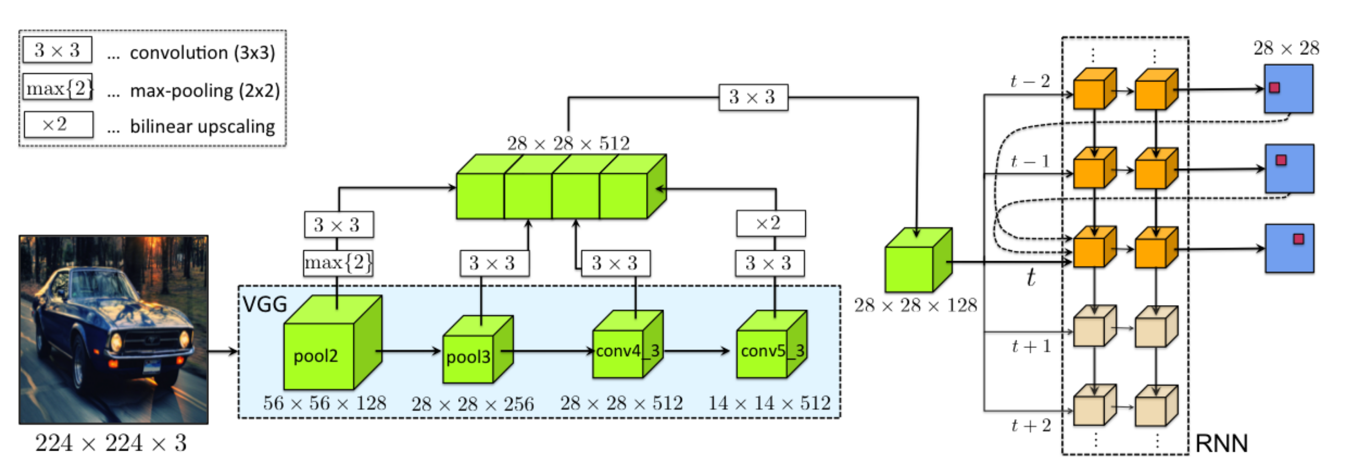
[Figure 1. Architecture of Polygon-RNN.]
Polygon-RNN has a VGG-16-like architecture as an encoder. The key modification is replacing the last Fully Connected (FC) and pooling layers with skip-connected convolutional layers to aggregate encodings of different granularity. The RNN decoder is a two-layer Convolutional LSTM (ConvLSTM) with skip connections from the previous two time steps. The decoder is responsible for the sequential prediction of polygon vertices. Figure 1 illustrates the architecture of the Polygon-RNN model.
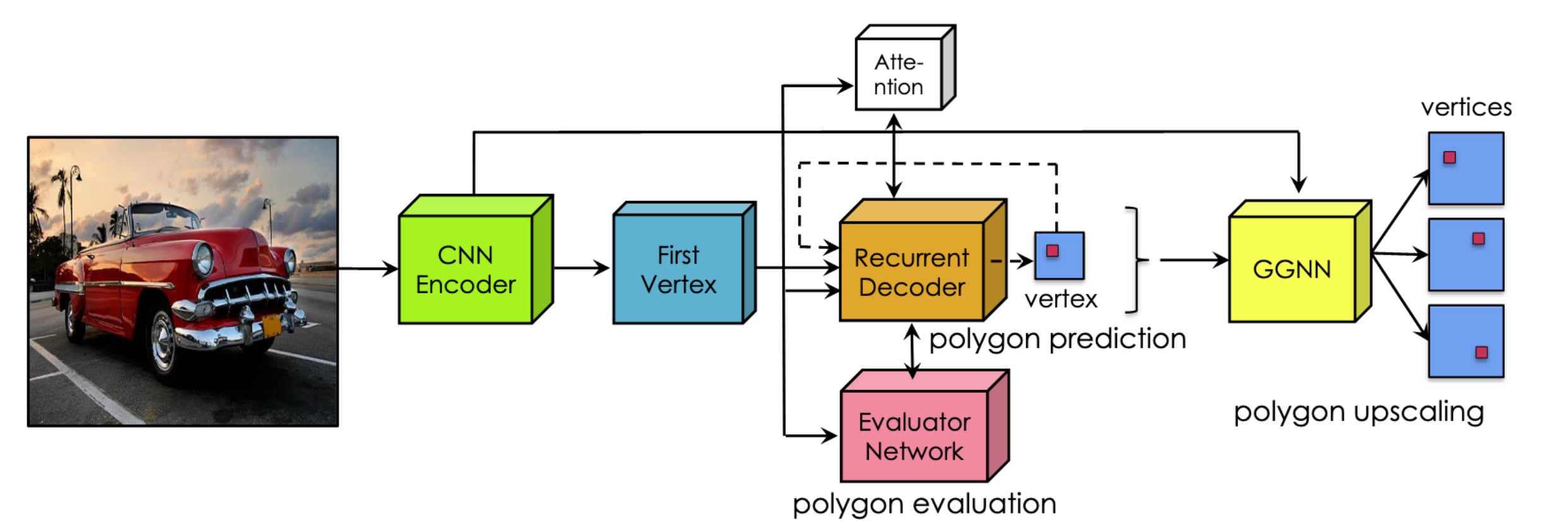
[Figure 2. Architecture of Polygon-RNN++.]
Polygon-RNN++
Improving upon its predecessor, Polygon-RNN++ (Acuna et al., 2018) was introduced the following year and included a series of upgrades. The new CNN encoder uses a ResNet-50-like structure and produces image features used to generate a set of first vertices. This encoder, unlike others, does not perform repeated downsampling in the CNN layers. Instead, they follow DeepLab (Chen et al., 2016) to introduce dilation with a reduced convolution stride to retain the large receptive field at the final layer. Although the RNN decoder remains a two-layer ConvLSTM, a new attention mechanism has been added atop it. The attention helps the RNN focus on a small neighborhood at each step, drastically increasing its performance. At the same time, the evaluator network will choose the most sensical polygon prediction computed from the different first vertex proposals. Finally, a new Gated Graphical Neural Network (GGNN) block was added to the architecture to help the model recover object instance segmentation vertices to the input image resolution.
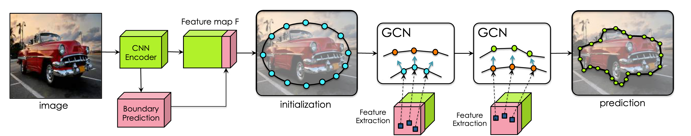
[Figure 3. Architecture of Curve-GCN.]
Curve-GCN
The Curve-GCN (Ling et al., 2019) formulation takes another step forward by discarding the sequential natured CNN-RNN formulation and uses a Graph Convolutional Network (GCN) to predict all the segmentation polygon vertices simultaneously, making it much more scalable with respect to the number of vertices. While the previous two works can only parametrize object outlines as polygons, Curve-GCN can also parametrize the outline with splines. The support for spline parameterization makes Curve-GCN efficient and precise towards approximating shapes with curvature. An outstanding choice is that the authors used the Centripetal Catmull-Rom spline (CRS) (Yuksel et al., 2011) instead of other common splines. In CRS, the control points will be on the calculated spline, making it more natural for inexperienced annotators. Figure 3 illustrates the Curve-GCN architecture.
Performance
These three works spanned the three consecutive years, 2017 to 2019, and achieved vast improvements in accuracy and efficiency each year. We defer the complete comparison to the papers and highlight a few comparisons instead. We focus on two metrics for the two polygon-based models: (1) speed up, in terms of mouse clicks, in interactive mode, and (2) IoU agreement with ground truth segmentation in automatic mode. On the other hand, Curve-GCN’s main improvement is code running time, thanks to its regressive prediction formulation, and we shall use running wall-clock time as a measurement.
In Polygon-RNN, the authors compared its performance against human annotators and found that the system results in a 4.7x speed up averaged across all classes in the challenging Cityscape dataset. In addition, the system achieves an approx. 80% IoU agreement with ground truth labels running in automatic mode. The improved Polygon-RNN++ was compared to its predecessor, Polygon-RNN. The authors found that it further delivers 2x click speed up in interactive mode and a 10% absolute increase in mean IoU in automatic mode. Curve-GCN achieves a slightly better automatic mode mean IoU on the CityScape dataset than Polygon-RNN++; however, it attains a drastic 10x and 100x wall clock runtime improvement compared to Polygon-RNN++.
Contour Based Approach
In this survey, we will focus on Deep Extreme Level Set Evolution, but we also want to mention the contour-based approach’s evolution. This line of work to object instance annotation aims to trace closed contours. The oldest techniques are based on level sets. Caselles et al. (1995) proposed a scheme for detecting object boundaries. It is based on active contours evolving in time according to intrinsic geometric measures of the image. This approach utilizes the relation between active contours and the computation of geodesics or minimal distance curves to produce accurate and regularized boundaries. In (Acuna et al., 2019), the authors use level set evolution with a carefully designed neural network for boundary prediction to find accurate object boundaries from coarse annotations. This design speeds up the annotation process drastically because annotators are only required to get coarse labeling. In DELSE (Wang et al., 2019), the authors revived using a level set for segmentation (Osher & Sethian, 1988; Caselles et al., 1995) by combining it with a CNN encoder structure that predicts level set evolution parameters.
DELSE
In the architecture pictured below, extreme boundary points are encoded as a heat map and concatenated with the image. Then, it will be passed to the encoder CNN. A multi-branch architecture predicts the initial level set function (a rough estimation through Level Set Branch) and evolution parameters (Motion Branch & Modulation Branch) used in level set evolution. Then DELSE evolves the initially estimated contour by iteratively updating the level set function.
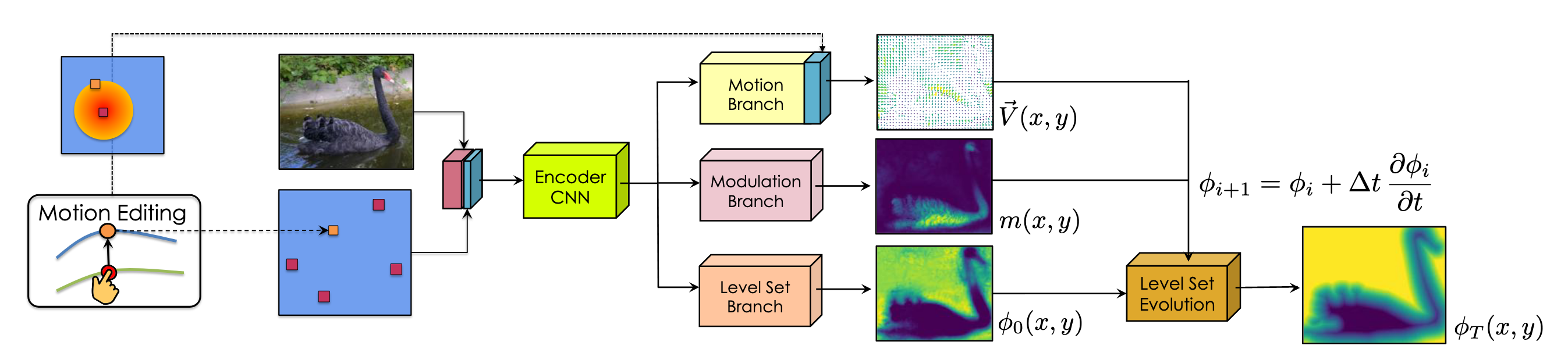
[Figure 4. Architecture of DELSE.]
Initial Level Set Function Prediction
Traditionally, we need a manual rough boundary to initialize the level set function, which is time-consuming. In DELSE, this initialization is much more efficient, taking four extreme points as input and utilizing the CNN model to generate a rough estimation of the initial level set function. Then, the model places a Gaussian around each extreme point and concatenates the RGB image as the fourth channel. The fourth channel input is propagated through an encoder CNN, and the extracted feature map is fed into the Level Set Branch to regress to the initial level set function.
DELSE Components
The level set evolutions consist of several updated terms. We can divide these updated terms into two categories: (1) External terms that attract the curve to the desired location and (2) Internal regularization terms on the curve’s shape.
However, in DELSE, the authors carefully designed three terms that best exploit deep neural networks to perform efficient level set evolution. (1) Motion Term. They feed the feature map into the Motion Branch to predict the motion map. The motion map consists of a vector at each pixel and forms a vector field indicating the direction and magnitude of the motion of the curve. (2) Curvature Term. We can regularize the predicted curve by moving it in the direction of its curvature. However, applying regularization directly on shapes with sharp corners would drastically decrease the model’s performance. The authors used Modulation Branch to predict a modulation function that selectively regularizes the curve to mitigate this. This design gave the model flexibility and power to preserve the real sharp corners around the object and only remove the noise that damages the shape of the curve. (3) Regularization term. During the evolution of the level set function, irregularities may occur and cause instability. The authors take the remedy method proposed by (Li et al., 2010) and introduce the distance regularization term to restrict the behavior of the level set function.
Performance
Compared to Polygon-RNN++, which predicts a single polygon around the object, the DELSE can handle objects with multiple components thanks to its level-set-based formulation. In addition, the object instance segmentation boundaries are continuously improved throughout the curve evolution process. Most noteworthily, the model can escape from flawed segmentation boundaries. Quantitatively, DELSE consistently outperforms Polygon-RNN++ in automatic mode in terms of IoU across all categories on the CityScape dataset and achieves 2%+ relative mean IoU improvement (from 71.38% to 73.84%).
Deformable Grid Approach
Gao et al. (2020) proposed DefGrid, which uses a deformable 2-dimensional triangular grid to outline objects. They employ a deep neural network to predict the grid offset parameters and argue that their method is more efficient than the traditional fixed uniform grid representation.
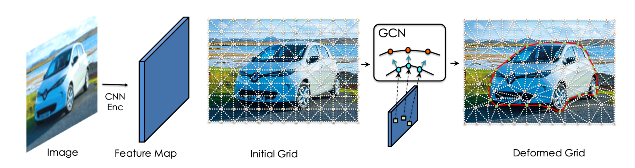
[Figure 5. The Deformable Grid (Def-Grid) Model.]
Deformable Grid
The DefGrid is a 2-dimensional triangular grid defined on an image plane. The primary grid consists of 3 vertices, each with a location that positions the triangle in the image. The Edges of triangles represent line segments and not self-intersect across triangles. The grid’s topology is fixed and does not depend on the input image. The DefGrid would deform the grid depending on the different input images. It deforms a triangular grid with uniformly initialized vertex positions to better align with image boundaries. The grid is deformed via a neural network and ensures no self-intersections happen. The intuition is that when the grid edges align with image boundaries, the pixels inside each grid cell have a minimal variance of RGB values. To utilize deep learning, the authors aim to minimize the variance in a differentiable way with respect to the position of the vertices.
Applications
We highlight the versatility of DefGrid as it supports many computer vision tasks that are done on fixed image grids. DefGrid can be inserted and served instantly for several levels of processing. For example, as an input layer, DefGrid can replace standard pooling methods by treating it as a learnable geometric downsampling layer. We will talk about two applications related to DefGrid.
(1) Learnable Geometric Downsampling. Typically, semantic segmentation requires high-resolution images as input and produces high-dimensional feature maps. Current deep CNNS often use feature pooling or other bottleneck structures to release the memory usage. We can use DefGrid to replace feature pooling and preserve finer geometric information. Moreover, usage like this has minimal technical overhead. The user only needs to insert a DefGrid using a shallow CNN encoder to predict a deformed grid, as illustrated in Figure 6.
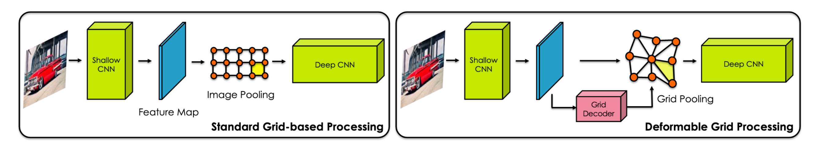
[Figure 6. Feature pooling in fixed grids versus DefGrid.]
(2) Object Mask Annotation. As Figure 7 shows, DefGrid supports predicting a pixel mask, outlining the boundary with a polygon/spline approach, and improving them via polygonal grid-based reasoning.
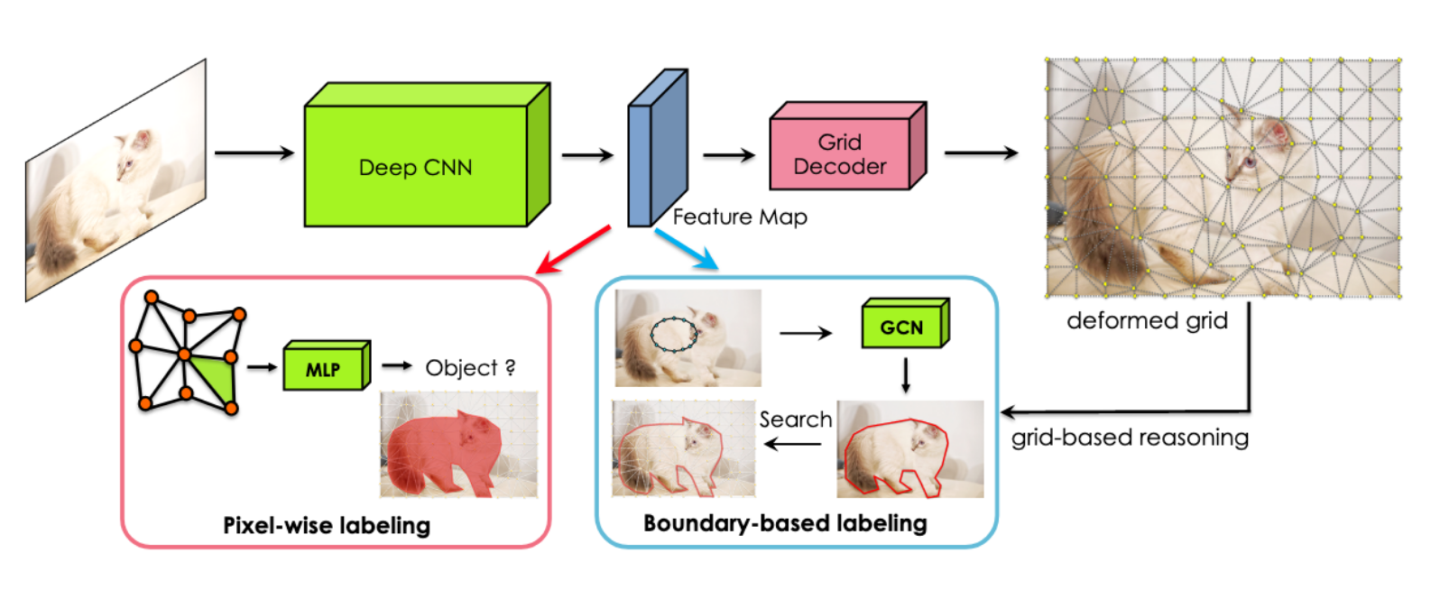
[Figure 7. Object mask annotation by reasoning on a DefGrid’s boundary aligned grid.]
Performance
The authors test the DefGrid instance segmentation model on the Cityscapes dataset for object annotation. They assume the annotator provides each object’s bounding box, and the task is to trace the object’s boundary. They use the image encoder from DELSE and add three branches to predict grid deformation, Curve-GCN points, and Distance Transform energy map. As shown in Figure 8, DefGrid consistently outperforms, over all categories, its predecessor Curve-GCN in terms of IoU. In addition, DefGrid achieves the highest F-measure scores when compared to other models. In particular, its performance can surpass the most expressive pixel-wise models, strongly indicating the importance of reasoning on the grid.
[Figure 8. Boundary-based object annotation on Cityscapes-Multicomp.]
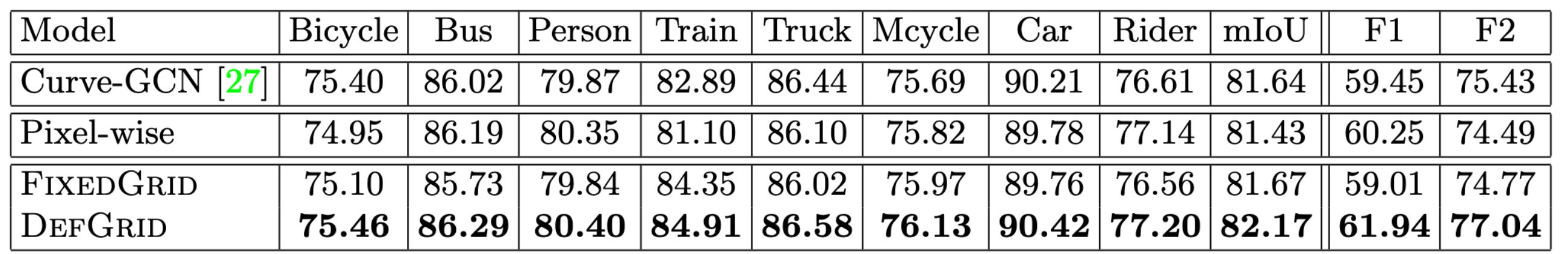
The authors also compare the performance between FixedGrid and DefGrid, as Figure 9 shows, where DefGrid achieves superior performance. The authors attribute the performance gains to better alignment with boundaries and more flexibility in tracing a longer contour.
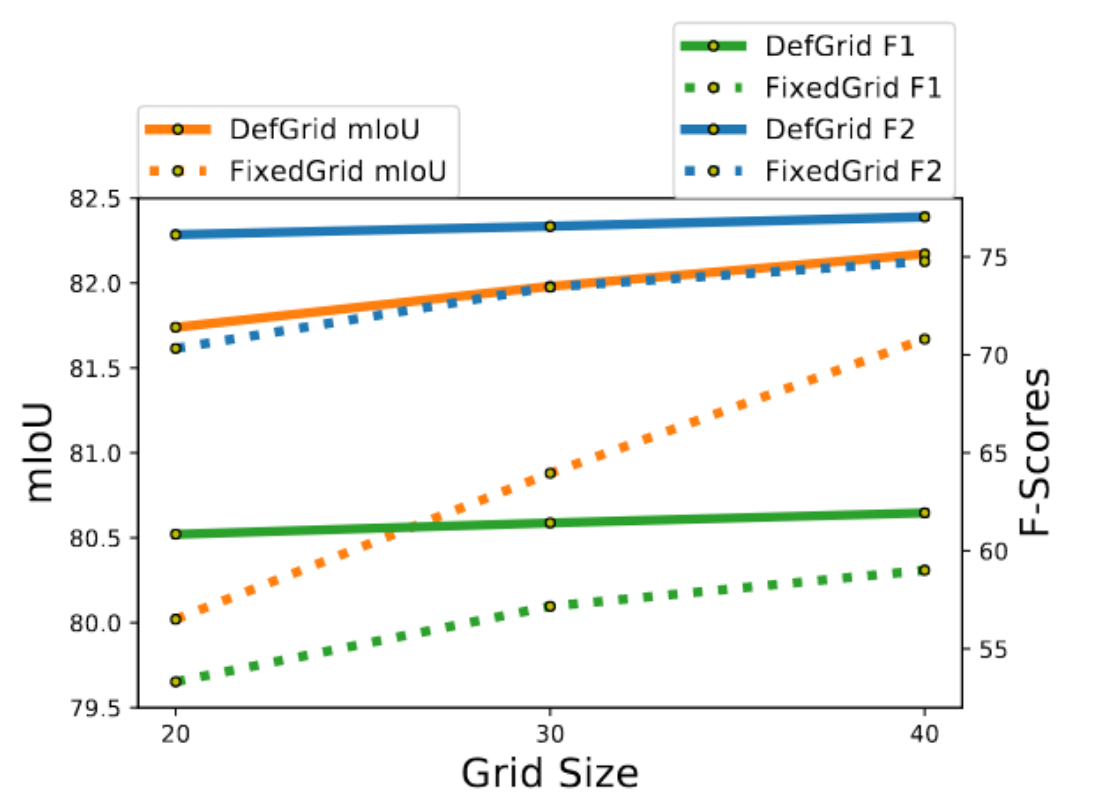
[Figure 9. Object annotation for Cityscapes: FixedGrid vs DefGrid.]
Beyond Single Still 2D Image: Adding Another Axis.
We briefly examine scribble-aided approaches that go beyond the width-height axes 2D still image setting by considering an additional axis as part of the most recent works in the suite. In this category, Scribble3D (Shen et al., 2020) considers the addition of a depth axis, predicting 3D object instance segmentation using scribbles drawn over a 2D projection. On the other hand, ScribbleBox (Chen et al., 2020) studies the addition time axis and allows video object instance segmentation.
Scribble3D
As shown in Figure 10, Scribble3D (Shen et al., 2020) is an interactive framework for annotating 3D object geometry from point clouds and RGB models. This framework enables a graphic non-specialist to produce good quality 3D meshes that fit 3D observations through an interactive learning-based approach. This annotation framework is composed of two stages. First, it produces an initial guess of the 3D mesh, and then it uses the 2D interface to correct the 3D error by scribbling in one or several desired 2D views. These manual scribbles are then fed into the neural architecture to generate an improved prediction of the 3D shape. For the final fine-grained meshes, the user can make edits to the 3D vertices of the object mesh directly.
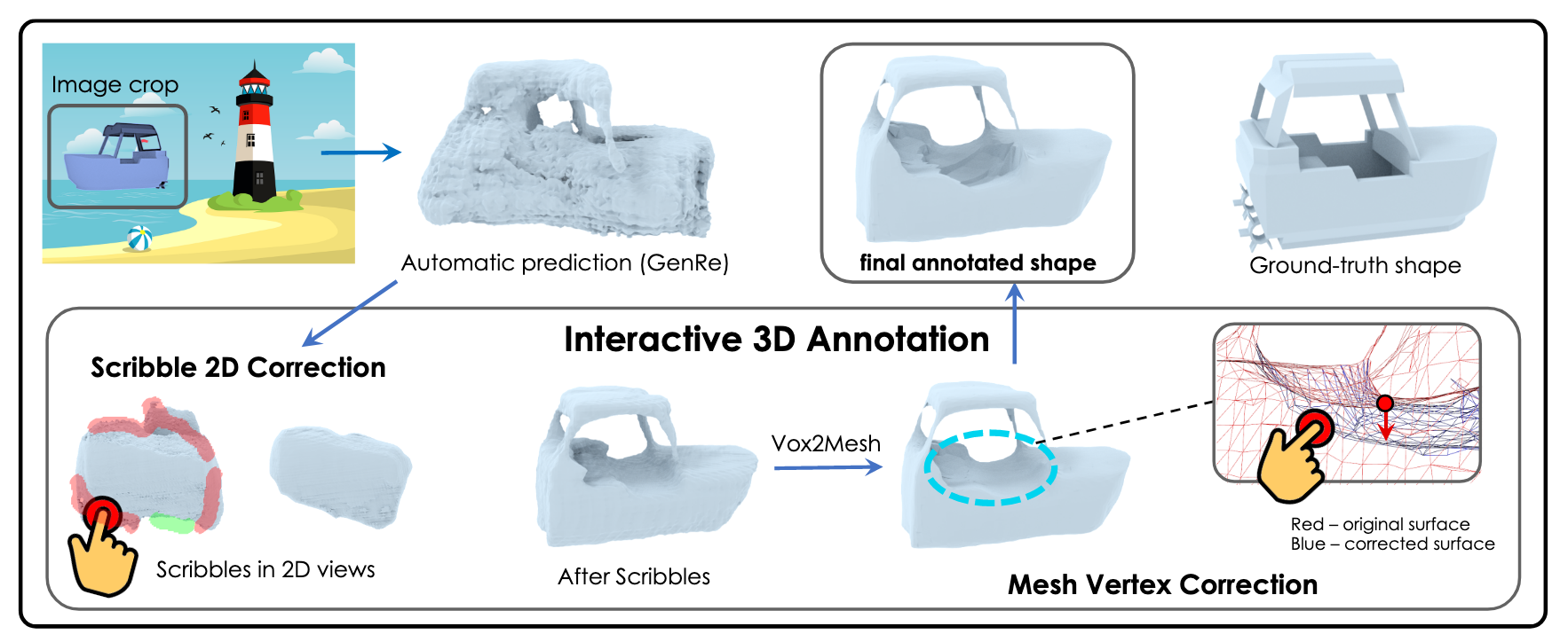
[Figure 10. Scribble3D: An interactive 3D annotation framework.]
ScribbleBox
ScribbleBox is a model (Chen et al., 2020) for interactive annotation of object instances in videos. The authors proposed to split the segmentation into two more straightforward tasks: annotating and tracking a loose box around each object across frames and segmenting the object in each tacked box.
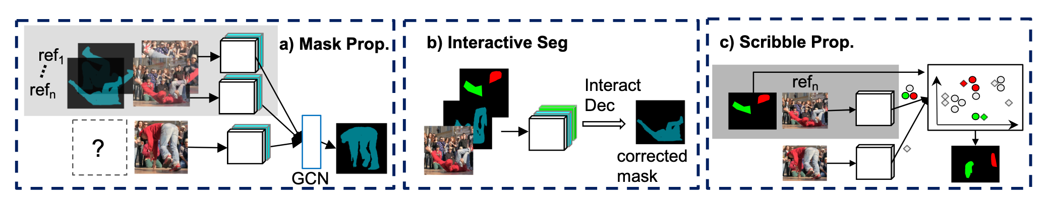
[Figure 11. Building blocks for Scribble-Box: An interactive framework for annotating object masks in videos.]
Figure 11 illustrates the three main building blocks for ScribbleBox. In (a), the mask propagation module predicts object masks for subsequent video frames given results from previous time steps. The interactive segmentation module in (b) can take in user scribble as input and generate a corrected mask for a frame. Notice that the model supports two types of errors: false positive and false negative, and expects users to annotate them with red and green, respectively. Last but not least, (c) propagates the correction to nearby frames, closing one loop of interaction.
Concluding Remarks
This survey took a chronological look at the various methods proposed for object instance segmentation and annotation via non-pixel-wise methods. We started from the polygon-based methods that used CNN-RNN structures. A strong emphasis was placed on using polygon boundaries, the most natural sparse representation that humans can correct. With the increasing popularity of Graph Neural Networks (GNN) variants, Curve-GCN discarded the recurrent formulation entirely and used a GCN to predict all boundary points directly and simultaneously. It is worth noting that Curve-GCN improved the code run time significantly. The latter two methods utilized contour and deformable grids to represent the boundaries, and each achieved state-of-the-art results at the time of publication. Finally, we briefly looked at the newest works in the Toronto Annotation Suite, namely Scribble3D and ScribbleBox, which handle data with an additional axis: depth and time.
It remains challenging for models to generate boundaries in a messy scene, even with the help of rough bounding boxes supplied by the human annotator. Recent advances in vision language models can project natural language input and vision signals into a common feature space. We expect to see methods that utilize these vision language models, via possibly an optional natural language description, to aid the automatic segmentation and annotation.
References
Acuna, D., Kar, A., & Fidler, S. (2019). Devil is in the Edges: Learning Semantic Boundaries from Noisy Annotations. CVPR. https://arxiv.org/abs/1904.07934
Acuna, D., Ling, H., Kar, A., & Fidler, S. (2018). Efficient Annotation of Segmentation Datasets with Polygon-RNN++. CVPR. https://arxiv.org/abs/1803.09693
Barriuso, A., & Torralba, A. (2012). Notes on image annotation.
Benenson, R., Popov, S., & Ferrari, V. (2019). Large-scale interactive object segmentation with human annotators. CVPR. https://arxiv.org/abs/1903.10830
Caselles, V., Kimmel, R., & Sapiro, G. (1995). Geodesic Active Contours. International Journal of Computer Vision 22(1), 61–79. https://www.cs.technion.ac.il/~ron/PAPERS/CasKimSap_IJCV1997.pdf
Castrejon, L., Kundu, K., Urtasun, R., & Fidler, S. (2017). Annotating Object Instances with a Polygon-RNN. CVPR. https://ieeexplore.ieee.org/document/8099960
Chen, B., Ling, H., Zeng, X., Gao, J., Xu, Z., & Fidler, S. (2020). ScribbleBox: Interactive Annotation Framework for Video Object Segmentation. ECCV. https://arxiv.org/abs/2008.09721
Chen, L.-C., Papandreou, G., Kokkinos, I., Murphy, K., & Yuille, A. L. (2016, April). DeepLab: Semantic Image Segmentation with Deep Convolutional Nets, Atrous Convolution, and Fully Connected CRFs. T-PAMI, 40(4):834–84. https://arxiv.org/abs/1606.00915
Gao, J., Wang, Z., Xuan, J., & Fidler, S. (2020). Beyond Fixed Grid: Learning Geometric Image Representation with a Deformable Grid. ECCV. https://arxiv.org/abs/2008.09269
Li, C., Xu, C., Gui, C., & Fox, M. D. (2010). Distance Regularized Level Set Evolution and Its Application to Image Segmentation. IEEE. https://ieeexplore.ieee.org/document/5557813
Ling, H., Gao, J., Kar, A., Chen, W., & Fidler, S. (2019). Fast Interactive Object Annotation with Curve-GCN. CVPR. https://arxiv.org/pdf/1903.06874.pdf
Osher, S., & Sethian, J. A. (1988). Fronts Propagating with Curvature Dependent Speed: Algorithms Based on Hamilton-Jacobi Formulations. Journal of Computational Physics, 79, pp.12-49. https://math.berkeley.edu/~sethian/Papers/sethian.osher.88.pdf
Russell, B. C., Torralba, A., Murphy, K. P., & Freeman, W. T. (2008). LabelMe: a database and web-based tool for image annotation. CVPR. https://www.cs.ubc.ca/~murphyk/Papers/labelmeIJCV08.pdf
Shen, T., Gao, J., Kar, A., & Fidler, S. (2020). Interactive Annotation of 3D Object Geometry using 2D Scribbles. ECCV. https://www.cs.toronto.edu/~shenti11/scribble3d/
Sun, X., Christoudias, C. M., & Fua, P. (2014). Free-Shape Polygonal Object Localization. ECCV. https://infoscience.epfl.ch/record/200244?ln=en
Tzutalin. (2015). LabelImg. Git code. https://github.com/tzutalin/labelImg
Wang, Z., Acuna, D., Ling, H., Kar, A., & Fidler, S. (2019). Object Instance Annotation with Deep Extreme Level Set Evolution. CVPR. https://www.cs.toronto.edu/~zianwang/DELSE/zian19delse.pdf
Yuksel, C., Schaefer, S., & Keyser, J. (2011). Parameterization and applications of Catmull–Rom curves. Computer-Aided Design 43(7):747-755. https://www.sciencedirect.com/science/article/pii/S0010448510001533?via%3Dihub
Zhang, Z., Fidler, S., Waggoner, J., Cao, Y., Dickinson, S., Siskind, J. M., & Wang, S. (2012). Superedge Grouping for Object Localization by Combining Appearance and Shape Information. CVPR. https://engineering.purdue.edu/~qobi/papers/cvpr2012.pdf
Zhou, B. (2020, 5 17). Yu Yi Fen Ge Gai Ru He Zou Xia Qu [How to go about semantic segmentation?]. Retrieved 6 3, 2022, from https://www.zhihu.com/question/390783647/answer/1226097849
Zhou, B., Zhao, H., Puig, X., Fidler, S., Barriuso, A., & Torralba, A. (2017). Scene Parsing through ADE20K Dataset. CVPR. https://people.csail.mit.edu/bzhou/publication/scene-parse-camera-ready.pdf