ASL Fingerspelling

We evaluate and compare 3 different implementations of Continuous Sign Language Recognition (CSLR): MiCT-RANet, a spatio-temporal approach, C2ST, which takes advantage of textual contextual information, and Open Pose landmarks. We implement the MiCT-RANet approach for ASL fingerspelling recognition and attempt to train it from scratch.

• Introduction
• Deep Learning Implementations
  • 1. MiCT-RANet
  • 2. C2ST
  • 3. OpenPose
• MiCT-RANet Implementation Details
• References

Introduction

250,000 to 500,000 people use American Sign Language (ASL) in the US, making it the third most commonly used language after English and Spanish. ASL interpretation is important because it removes barriers to communication for deaf or hearing-impaired people, allowing more interactions between them and hearing people who do not know ASL. It also expedites communication during emergency situations by removing the need for an interpreter, and provides alternative accessibility options for smart home devices and mobile applications.

There are 5 components to a sign language: hand shape, location, movement, orientation, and non-manual. Non-manual components include facial expressions and slight nuances not directly measured through hand position that add meaning to the phrase, and often is the distinction between different words that have the same sign [10].

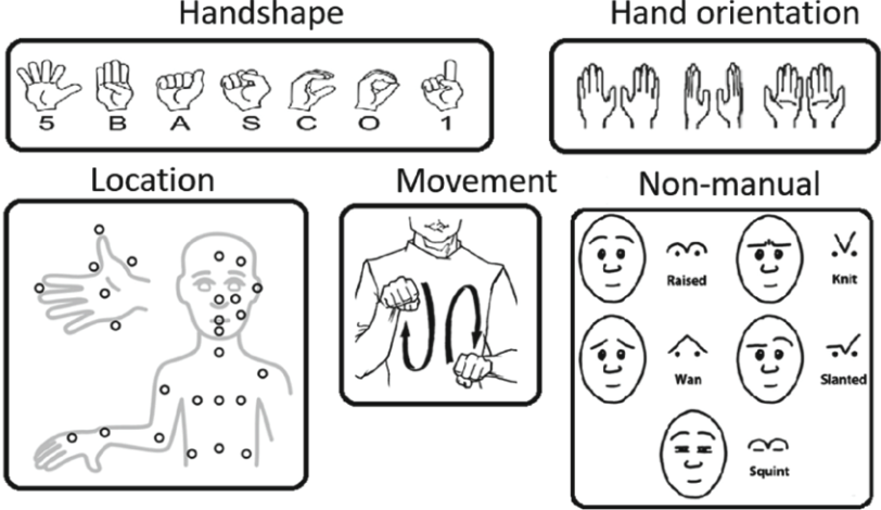Figure 1: Components of Sign Language [10]

The scope of our project will be to extract words and phrases from fingerspelling for ASL which uses hand shape, orientation, and movement, especially letters that include moving parts. We will take as input short video sequences and classify them live, returning as output the prediction of the word, letter-by-letter. We will use the dataset called Chicago Fingerspelling in the Wild(+) which includes 55,232 fingerspelling sequences signed by 260 signers [6].

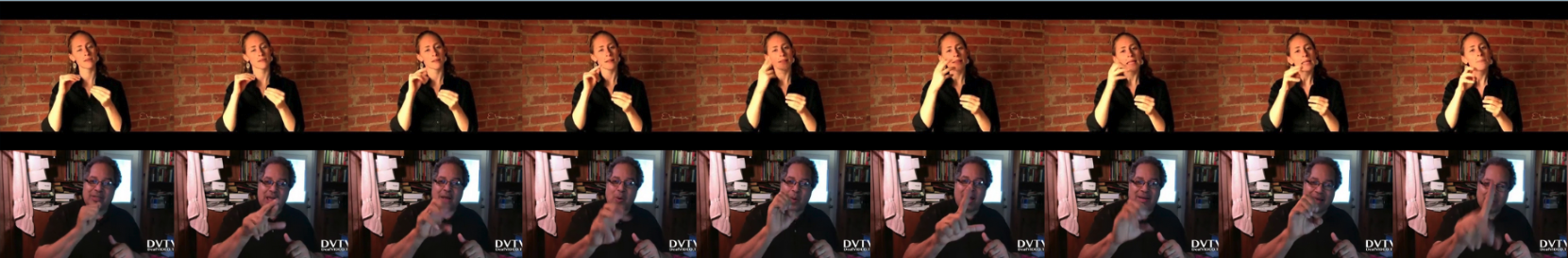Figure 2: Sample fingerspelling frame sequences taken from ChicagoFSWild+ dataset [6]

We evaluate and compare 3 different implementations of Continuous Sign Language Recognition (CSLR): MiCT-RANet, a spatio-temporal approach, C2ST, which takes advantage of textual contextual information, and Open Pose landmarks. We implement the MiCT-RANet approach and attempt to train it from scratch. Our code can be found here.

Deep Learning Implementations

1. MiCT-RANet

MiCT-RANet embodies the conventional CSLR approach of chaining a spatial module and a temporal module, followed by Connectionist Temporal Classification. We discuss each component in the following sections.

Part 1: MiCT

In 3D convolutions, kernels slide along spatial and temporal dimensions of the input to make 3D spatio-temporal feature maps. The tensor size: T x H x W x C which stands for temporal duration, height, width, number of channels respectively. The output is T' x H' x W' x N where N=number of filters. See figure 3 for diagram. The main problem with 3D convolutions are that they can be difficult to optimize with high memory usage and cost. The solution in this approach by Zhou et al. [8] is a Mixed Convolution with 2D and 3D CNNs. MiCT is mixed in 2 ways, first by concatenating connections and adding cross-domain residual connections (see figure 4). The input is passed through a 2D convolution to extract static features then put through a 3D convolution and a cross-domain residual so the 3D convolution only needs to learn residual information along the temporal dimension. This reduces the total number of 3D convolutions needed, reducing model size, while maintaining high performance. Compared to other models like C3D which uses 8 3D convolutions, MiCT uses 4 3D convolutions with better performance and lower memory usage. Below is code for the forward pass of a single MiCT block:

def forward(self, x):
        if self.t_padding == 'forward':
            out1 = F.pad(x, [1, 1, 1, 1, 0, 2*(self.mict_3d_conv_depth//2)], 'constant', 0)
            out1 = self.conv(out1)
        else:
            out1 = self.conv(x) # 3D convolution
        out1 = self.bn(out1)
        out1 = self.relu(out1)

        x, depth = _to_4d_tensor(x, depth_stride=self.stride[0])
        out2 = self.bottlenecks[0](x) # 2D convolution block on first timestamp (eg. inception, resnet etc.)
        out2 = _to_5d_tensor(out2, depth)
        out = out1 + out2 # concat

        out, depth = _to_4d_tensor(out)
        for i in range(1, self.blocks):
            out = self.bottlenecks[i](out) # final 2D convs
        out = _to_5d_tensor(out, depth)

        return out

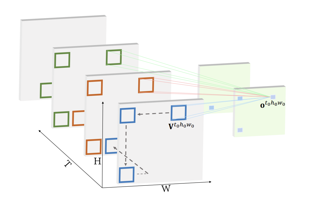Figure 3: Visualization of a 3D Convolution by Zhou et al.[8]

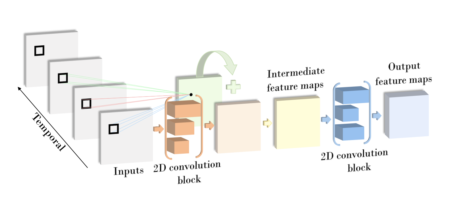Figure 4: Illustration of the cross-domain residual connection used in MiCT developed by Zhou et al.[8]

Part 2: RANet

RANet is short for “Recurrent Attention Network”. The RANet can be modeled as a function that takes a sequence of \(T\) input images (in the space \(I\)) and outputs a sequence of \(T\) temporal image features encoded in its hidden state \(E\): \(f: I^T \to E^T\). As we have learned in class, a recurrent neural network contains a hidden state \(e_t\) at each time \(t\). This hidden state is used in conjunction with the input at time \(t\) to compute the inference. The hidden state is also updated at each time step to \(e_{t + 1}\). In the paper referenced by MiCT-RANet, Shi et. al [6] used the LSTM algorithm to update the hidden state.

We will briefly overview the standard LSTM algorithm. In addition to the hidden state \(e_t\), LSTM also incorporates a cell state \(C_t\) which helps it retain long-term context, denoted in this paper as \(h_t\). Within an LSTM cell, at each time step the cell state, hidden state, and input interact via three gates: the forget gate, input gate, and output gate. The forget gate uses the hidden state and input to selectively erase components of the cell state. This allows the LSTM cell to forget irrelevant context. The input gate adds a combination of the hidden state and input to the cell state. This allows the LSTM cell to retain new context. Finally, the output gate uses a combination of the new cell state, hidden state, and input to compute the next hidden state. From this architecture, we can see that the cell state acts as a sort of long term memory that the LSTM cell can erase and read from at different time steps.

In addition to a recurrent neural network, Shi et. al also uses spatial attention to compute the relevant parts of the image. The problem with fingerspelling recognition is that the hand which we want the model to focus on is usually only a tiny fraction of the entire image. Spatial attention allows us to highlight the relevant part of the image and attenuate the irrelevant parts. Spatial attention depends on the hidden state \(e_t\) as well as the input feature map \(f_t\). The spatial attention formula is given as follows:

Subscript \(t\) represents the time step. \(v_{tij}\) are the alignment scores, while \(\beta_{tij}\) is the attention map, which is then used to update the cell state \(h_t\). Shi et. al then optionally augments this vanilla spatial attention with a “prior-based attention term”, which is essentially another map of the relevant locations on the feature map. For example, they recommend an optical flow map, which would boost the attention of regions of motion, which are likely to be the hands. The augmentation process is essentially a normalized dot product.

We have seen how Shi et. al combines LSTM-based recurrent neural networks with spatial attention to achieve an architecture known as RANet. Their paper also uses the technique of iterative attention to improve their model. Iterative attention is essentially training multiple RANet models on iteratively zoomed-in images. The point of this technique is to allow the latter models to better focus on the hand. Using multiple models allows different models to focus on differently-sized details and yields better results. See the flow diagram of RANet, and along with the code for the forward pass below:

def forward(self, hidden, feat_map, prior_map):
        """
        Forward pass for one step of the recurrent attention module.

        :param hidden: LSTM's latest hidden state with shape:
            ([batch_size, hidden_size], [batch_size, hidden_size]), ie ([1, 512], [1, 512])
        :param feat_map: feature maps of the current frame with shape:
            [h_map * w_map, batch_size, n_channels], ie. [196, 1, 512]
        :param prior_map: the spatial attention prior map of the current frame with shape:
            [h_map * w_map, batch_size], ie. [196, 1]
        :return: the new hidden state vector
        """
        H = self.hidden_size
        N, B, C = list(feat_map.size())  # number of pixels, batch size and number of channels

        query = torch.matmul(hidden[0], self.Wh)
        key = torch.matmul(feat_map.view(-1, C), self.Wk).view(N, B, H)
        value = torch.matmul(feat_map.view(-1, C), self.Wv).view(N, B, C)

        scores = torch.tanh(query + key).view(-1, H)
        scores = torch.matmul(scores, self.v).view(N, B)
        scores = F.softmax(scores, dim=0)
        attn_weights = scores * prior_map

        context = (attn_weights.view(N, B, 1).repeat(1, 1, C) * value).sum(dim=0)  # [B, C] # value is a bit different from the equation; in the equation value is feat_map directly but we’ve multed a weight matrix
        sum_weights = attn_weights.sum(dim=0).view(B, 1).clamp(min=1.0e-5)  # [B, 1]
        return self.lstm_cell(context / sum_weights, hidden)

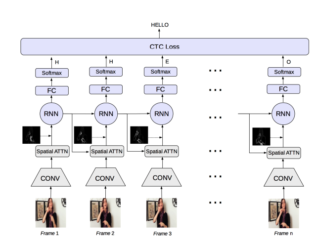Figure 5: Flow diagram of RANet by Shi et al.[6]

Part 3: Connectionist Temporal Classification

At inference time, the model generates a frame-by-frame letter sequence \(Z\) by passing the image features \(E\) through a language model and collapses it to prediction \(\hat{Y}\) via a label collapsing function \(\mathbb{B}\). This typically involves some combination of removing blanks and deduplication.

At train time, MiCT-RANet opts for an FC layer with softmax instead and optimizes the following loss function:

where \(P(Z \mid G) = \prod_sP(z_s \mid G)\). Intuitively, the loss is the negative log likelihood of summing all the possible alignments (aka frame-by-frame letter sequences) \(Z\).

Here is a diagram of the overall architecture of MiCT-RANet:

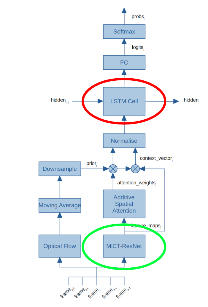Figure 6: Architecture diagram of MiCT-RANet

2. C2ST

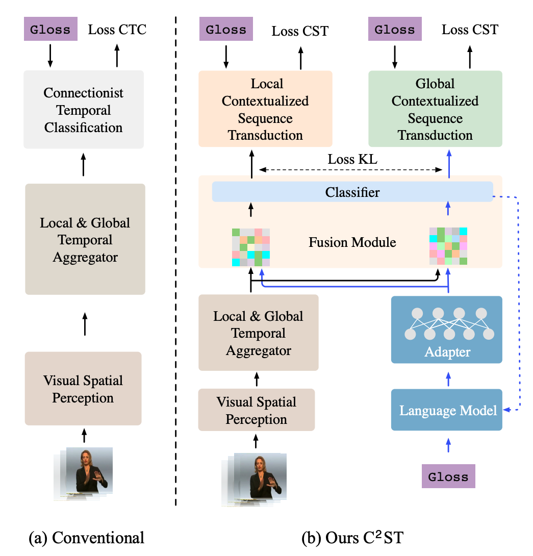Figure 7: Flow diagram of C2ST by Zhang et al.[7]

Zhang et. al [7] argue that conventional CSLR methods don’t take advantage of contextual dependencies between words. This is because the CTC loss makes an independence assumption between gloss tokens ¹. Recall the equation used to generate alignments \(Z\):

We see that each token \(z_s\) is generated independent of each other. To this end, they propose a framework that extracts and fuses contextual information from the text sequence with the spatio-temporal features, achieving SOTA performance of 17.7 WER ² on the Phoenix-2014 dataset [4]. Here is a general workflow (also see figure 7):

Let \(X = \{x_i\}_{i = 1}^N\) be the input video with \(N\) frames, which is divided into \(S\) chunks, and \(Z = \{z_i\}_{i=1}^S\) be the predicted alignment.

1. Pass \(X\) into the spatio-temporal module to obtain visual features \(L = \{l_s\}_{s = 1}^S\).
2. Let \(z_0 = \oslash\). For time step \(s\) in range \(\{1 .. S\}\):
   1. Feed gloss sequence generated so far \(Y_{<s} = \{y_i\}_{i = 0}^{s-1}\) into the language module to encode sequence feature \(b_{<s}\).
   2. Sum visual and sequence features \(l_s\) and \(b_{<s}\) to get fused feature \(j_s = l_s + b_{<s}\).
   3. Generate \(z_s\) by feeding \(j_s\) into the classifier and using a decoding algorithm (such as beam search).
3. The final step of training and inference proceeds the same way as in CTC. More details on the loss function in the “Loss Function Details” section.

Spatio-Temporal Module Details

The paper uses the Swin-Transformer pre-trained on ImageNet as the vision backbone for the spatial module, with window size \(7\) and output size \(768\). FOr the local temporal module, a 1D-TCN with Temporal Lift Pooling [9] with \(1024\) output dimension is used. Finally, a 2 layer Bi-LSTM is used for extracting global temporal features.

Language Module Details

The paper uses a pre-trained BERT-base as the language model, fine-tuned on the target gloss sequences in the CSLR train-set. An adaptor layer is used to account for the variance difference in gloss sequences and human grammar.

Loss Function Details

The paper uses a three-part loss function:

\(\mathcal{L}_{CST}\) is the negative log likelihood of the target sequence normalized by STC term:

Where \(p(Z \mid J) = \prod_s P(z_s \mid z_{<s}, J)\). Here, \(P(Z \mid J)\) is the probability of an alignment \(Z\) as estimated by the decoder, and summing up all possible alignment paths \(Z\) gives us the probability of the target sequence. The paper does this for the chunk and video levels (pass in local visual features $L$ for chunk level and global features \(G\) for video level), hence \(\mathcal{L}_{CST}^c, \mathcal{L}_{CST}^v\). The STC function is unspecified, but could be the edit distance between the ground-truth sequence \(Y\) and predicted sequence \(Z\) after removing the blanks. This helps pay more attention to potential sequences predicted by the model that have a smaller sequence-level error. Note that \(P(z_s \mid z_{<s}, J)\) breaks the independence assumption by conditioning the decoder model on the previous tokens \(z_{<s}\) as well.

\(\mathcal{L}_{KL}\) is a KL-divergence term to ensure consistency between chunk-level features \(J^c\) and video-level features \(J^v\).

3. OpenPose

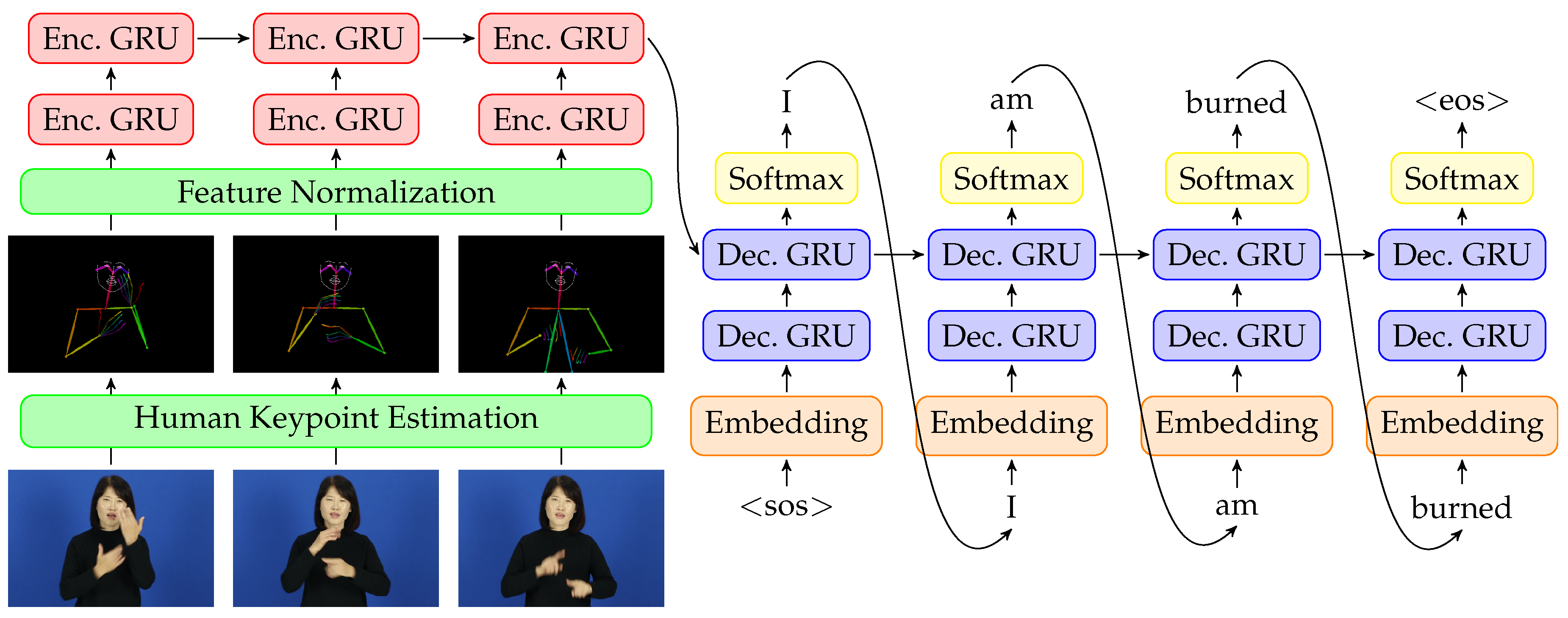Figure 8. A picture of the model architecture Ko et. al [3] developed from their paper

OpenPose is an open source 3D pose estimation system developed by researchers at CMU [11]. OpenPose employs a two-branch feature extraction architecture to accurately and efficiently construct pose keypoints. Here are some more details about the system:

1. Two-branch architecture to predict heatmaps and Part Affinity Fields (PAFs):
   1. Keypoint Detection Branch: this branch outputs heatmaps representing the likelihood of each keypoint (e.g., elbows, knees) being present at each pixel location.
   2. PAFs: this branch outputs vector fields that encode the orientation and association between pairs of keypoints (e.g., the direction from a shoulder to an elbow).
2. The base network (feature extractor, typically a CNN) processes the input image and produces feature maps, which are passed to subsequent stages.
3. Iterative Refinement (Cascaded Stages)
   1. The first stage generates initial heatmaps and PAFs using feature maps from the base network.
   2. Each subsequent stage refines the heatmaps and PAFs using the outputs from the previous stage and the original feature maps.
   3. The outputs converge to more accurate keypoint and PAF predictions as the stages progress.
4. OpenPose uses a dual loss function and the total loss is the sum of these losses across all stages.:
   1. Heatmap Loss (L2): Measures the difference between predicted and ground-truth heatmaps.
   2. PAF Loss (L2): Measures the difference between predicted and ground-truth PAFs.
5. After obtaining the heatmaps and PAFs, OpenPose uses a greedy bipartite matching algorithm to group detected keypoints into individual poses. This step connects keypoints based on their PAF values and geometric constraints.

Brock et al. [2] utilized OpenPose to recognize non-manual content in a continuous Japanese sign language with two main components. First, they used supervised learning to do automatic temporal segmentation with a binary random forest classifier, classifying 0 for transitions and 1 for signs. After frame wise label prediction and segment proposal, they used a segment wise word classification with a CNN, then translating those predicted segment labels to sentence translation.

Ko et al. [3] adapted OpenPose for the task of Korean Sign Language (KSL) recognition and translation. The paper’s primary contribution lies in its two-step pipeline. First, OpenPose was used to extract body and hand keypoints from video sequences of KSL, generating a structured skeleton representation of signers. Second, a custom temporal segmentation approach classified motion patterns into discrete signs. This segmentation was followed by a sequence-to-sequence model for translating the segmented signs into natural language sentences. The method was tested on a custom dataset of KSL videos.

MiCT-RANet Implementation Details

Training code and fine-tuned model weights were not given, so we had to train from scratch. Due to compute constraints, we were only able to train on 1000 sequences and validate on 981. Originally following the paper’s hyperparameters, we found that SGD with lr=0.01 and momentum=0.9 caused exploding gradients, so we switched to Adam with lr=0.001. However, the model would now consistently predict empty sequences, and we could not rectify that. It is likely that the model will need to be trained on much more data and undergo more careful hyperparameter finetuning to produce noteworthy results. You can find the code we used here.

References

[1] Redmon, Joseph, et al. “You only look once: Unified, real-time object detection.” Proceedings of the IEEE conference on computer vision and pattern recognition. 2016.

[2] Brock, H., Farag, I., and Nakadai, K. “Recognition of non-manual content in continuous Japanese sign language.” Sensors (Switzerland), vol. 20, no. 19, pp. 1–21, 2020.

[3] Ko, Sang-Ki, Chang Jo Kim, Hyedong Jung, and Choongsang Cho. “Neural Sign Language Translation Based on Human Keypoint Estimation.” Applied Sciences, vol. 9, no. 13, p. 2683, 2019. https://doi.org/10.3390/app9132683

[4] Koller, O., et al. “Continuous sign language recognition: Towards large vocabulary statistical recognition systems handling multiple signers.” Computer Vision and Image Understanding, 2015.

[5] Prikhodko, A., Grif, M., and Bakaev, M. “Sign language recognition based on notations and neural networks,” 2020.

[6] Shi, et al. “Fingerspelling recognition in the wild with iterative visual attention,” 2019.

[7] Zhang, H., et al. “C2ST: Cross-modal Contextualized Sequence Transduction for Continuous Sign Language Recognition.” 2023 IEEE/CVF International Conference on Computer Vision (ICCV), 2023.

[8] Zhou, et al. “MiCT: Mixed 3D/2D Convolutional Tube for Human Action Recognition,” 2018.

[9] Hu, L., et al. “Temporal lift pooling for continuous sign language recognition.” CoRR, 2022.

[10] Prikhodko, A., Grif, M., & Bakaev, M. “Sign language recognition based on notations and neural networks.” 2020.

[11] Cao, Z., et al. “OpenPose: Realtime Multi-Person 2D Pose Estimation using Part Affinity Fields.” IEEE Transactions on Pattern Analysis and Machine Intelligence, 2019.