Medical Image Segmentation

This report covers medical image segmentation using U-Net, U-NET++, and PSPNet. These models are ran on an ISIC challenge dataset from 2017.

• Introduction
• Dataset
• Evaluation Methods
  • Mean Dice Coefficient
  • Last Layer CAM
  • Middle Layer Grad-CAM
• Model 1: U-Net
  • Architecture
  • Training
  • Results
  • Discussion
• Model 2: U-Net++
  • Architecture
  • Code Implementation
  • Training
  • Results
  • Discussion
• Model 3: PSPNet
  • Architecture
  • Code Implementation
  • Training
  • Results
  • Discussion
• Conclusion
• Reference

Introduction

Medical image segmentation involves taking a medical image obtained from MRI/CT/etc. and segmenting different parts of the image. More specifically, given a 2D or 3D medical image, the goal is to produce a segmentation mask of the same dimension as the input. Labels in this mask correspond semantically to relevant parts of the image that are classified based on predefined classes. Some examples of classes include background, organ, and lesion.

Unlike normal image classification tasks or most image segmentation tasks, medical image segmentation requires a very high level of accuracy. Radiologists who work with these images are trained for years to be able to accurately segment these images and identify lesions accurately. However, there are many more medical images than doctors that can make accurate diagnoses in the world, and so medical image segmentation attempts to solve this problem. Essentially, medical image segmentation aims to assist radiologists in detecting lesions from medical image scans and identifying regions of interest in an organ, reducing the amount of time radiologists may take to annotate these images.

The models we will explore in this paper to implement this solution are U-Net, U-Net++, and PSPNet. The implementations of these models are inspired by existing codebases that implemented them. The results that come out of these models will be quantitatively evaluated using the IoU and DICE score metrics. In addition to this, to better aid in the visual understanding of how these images are segmented, we will implement Grad-CAM and CAM. These will show which regions of the input contributed to the model’s predictions at different layers of the model. We will apply Grad-CAM and CAM to U-Net.

Dataset

The dataset used for this paper comes from ISIC (International Skin Imaging Collaboration), specifically the ISIC challenge dataset from 2017 [1]. The training dataset consists of 2000 skin lesion images in JPEG format and 2000 superpixel masks in PNG format. The ground truth training data consists of 2000 binary mask images in PNG format, 2000 dermoscopic feature files in JSON format, and 2000 lesion diagnoses. The goal of this dataset was train models to accurately diagnose melanoma. The challenge using this dataset involved segmenting images, feature detection, and disease classification. For the purposes of this paper, we will only focus on segmenting medical images, meaning we will not be using the 2000 dermoscopic feature files and 2000 lesion diagnoses.

Evaluation Methods

To evaluate the architectures described in the three papers on a single dataset, we used the following metrics so our evaluation was consistent evaluation approach.

Mean IoU

Mean Intersection over Union (IoU) is the overlap between the predicted and ground truth segmentation masks over all test samples. Each IoU can be found by:

This gives a measure of the model’s segmentation accuracy.

Mean Dice Coefficient

Mean Dice coefficient is the similarity between the predicted and ground truth masks over all test samples and a single score can be found with:

The closer to 1 the better overlap.

Last Layer CAM

A Class Activation Map (CAM) shows the regions of the input that contributed most to the model’s predictions. In our usecase of medical image segmentation CAM shows areas where the model focuses for classifying pixels as lesion or non-lesion. We implemented this and applied it to our three architectures get a better idea of the model’s inner workings. Here is our implementation:

class CAM:
    def __init__(self, model, target_layer):
        self.model = model
        self.target_layer = target_layer
        self.activations = None
        # this is the important line
        self.target_layer.register_forward_hook(self.save_activations)

    def save_activations(self, module, input, output):
        self.activations = output

    def compute_cam(self, input_image):
        self.model.eval()
        output = self.model(input_image)
        activations = self.activations.cpu().detach().numpy()
        weights = np.mean(output.cpu().detach().numpy(), axis=(2, 3))
        cams = []
        for img_idx in range(input_image.shape[0]):
            cam = np.zeros(activations.shape[2:], dtype=np.float32)
            for channel_idx, weight in enumerate(weights[img_idx]):
                cam += weight * activations[img_idx, channel_idx]
            cam = np.maximum(cam, 0)
            cam = cam - np.min(cam)
            cam = cam / np.max(cam)
            cams.append(cam)
        return cams

Middle Layer Grad-CAM

A Gradient-weighted Class Activation Map (Grad-CAM) gives a detailed visualization of how a model’s inner layers respond to an input by using gradients from the model’s backward pass during inference (which is possible by adding a PyTorch hook). Here is our implementation:

class GradCAM:
    def __init__(self, model, target_layer):
        self.model = model
        self.target_layer = target_layer
        self.gradients = None
        self.activations = None
        # these are the important lines
        self.target_layer.register_forward_hook(self.save_activations)
        self.target_layer.register_backward_hook(self.save_gradients)

    def save_activations(self, module, input, output):
        self.activations = output

    def save_gradients(self, module, grad_input, grad_output):
        self.gradients = grad_output[0]

    def compute_cam(self, input_image, target_pixel=None):
        self.model.eval()
        output = self.model(input_image)
        if target_pixel is None:
            h, w = output.shape[2:]
            target_pixel = (h // 2, w // 2)
        self.model.zero_grad()
        target_value = output[0, 0, target_pixel[0], target_pixel[1]]
        target_value.backward()
        gradients = self.gradients.cpu().detach().numpy()
        activations = self.activations.cpu().detach().numpy()
        weights = np.mean(gradients, axis=(2, 3))
        cam = np.zeros(activations.shape[2:], dtype=np.float32)
        for i, w in enumerate(weights[0]):
            cam += w * activations[0, i]
        cam = np.maximum(cam, 0)
        cam = cam - np.min(cam)
        cam = cam / np.max(cam)
        return cam

Model 1: U-Net

The earliest segmentation model we evaluated is U-Net, a convolutional neural network architecture designed specifically for biomedical image segmentation although today U-Net is being used for many different tasks.

Architecture

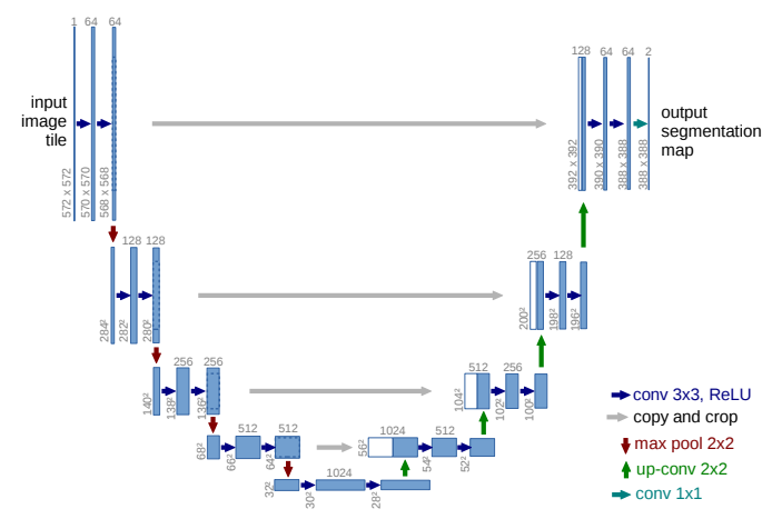
U-Net Architecture diagram from [2]

The most prominent features of U-Net’s architecture are its shape and its skip connections. The shape is a result of the two halves of the down and up-sampling process and the passing of feature maps directly to later convolution layers:

Encoder (Contracting Path)

• Captures global context by progressively reducing the spatial dimensions of the input while extracting deeper semantic features.
• At each down-sampling step, the spatial resolution is halved, and the number of feature channels is doubled through a 2x2 max pool operation.
• Deeper layers encode the overall structure and high-level semantics of the image.

class Encoder(nn.Module):
    def __init__(self):
        super(Encoder, self).__init__()
        self.enc1 = DoubleConv(3, 64)
        self.enc2 = nn.Sequential(
            nn.MaxPool2d(kernel_size=2, stride=2),
            DoubleConv(64, 128)
        )
        self.enc3 = nn.Sequential(
            nn.MaxPool2d(kernel_size=2, stride=2),
            DoubleConv(128, 256)
        )
        self.enc4 = nn.Sequential(
            nn.MaxPool2d(kernel_size=2, stride=2),
            DoubleConv(256, 512)
        )

    def forward(self, x):
        skip_connections = []
        x = self.enc1(x)
        skip_connections.append(x)
        x = self.enc2(x)
        skip_connections.append(x)
        x = self.enc3(x)
        skip_connections.append(x)
        x = self.enc4(x)
        skip_connections.append(x)
        return x, skip_connections

Decoder (Expanding Path)

• Restores the spatial resolution of the feature maps to reconstruct the segmentation mask.
• Uses 2x2 up-sampling convolutions to increase spatial dimensions and reconstruct the segmentation mask from encoded features.
• Combines deep, semantic features with fine-grained details to produce precise segmentation maps.

class Decoder(nn.Module):
    def __init__(self):
        super(Decoder, self).__init__()
        self.up4 = nn.Sequential(
            nn.ConvTranspose2d(1024, 512, kernel_size=2, stride=2),
            DoubleConv(1024, 512)
        )
        self.up3 = nn.Sequential(
            nn.ConvTranspose2d(512, 256, kernel_size=2, stride=2),
            DoubleConv(512, 256)
        )
        self.up2 = nn.Sequential(
            nn.ConvTranspose2d(256, 128, kernel_size=2, stride=2),
            DoubleConv(256, 128)
        )
        self.up1 = nn.Sequential(
            nn.ConvTranspose2d(128, 64, kernel_size=2, stride=2),
            DoubleConv(128, 64)
        )

    def forward(self, x, skip_connections):
        x = self.up4(torch.cat((skip_connections[-1], x), dim=1))
        x = self.up3(torch.cat((skip_connections[-2], x), dim=1))
        x = self.up2(torch.cat((skip_connections[-3], x), dim=1))
        x = self.up1(torch.cat((skip_connections[-4], x), dim=1))
        return x

Skip Connections

• Skip connections pass feature maps directly from the encoder to the decoder, bypassing the deeper layers of the network.
• Feature maps from the encoder are copied and cropped to match the dimensions of the decoder feature maps (to address size mismatches caused by up-sampling). These are then concatenated with the decoder feature maps.
• This allows the model to retain high-resolution spatial details that are typically lost during down-sampling.

Down-Up Connection

• To connect the above implemenations of the encoder and decoder we can add a layer to bridge the two.

class Bottleneck(nn.Module):
    def __init__(self):
        super(Bottleneck, self).__init__()
        self.bottleneck = DoubleConv(512, 1024)

    def forward(self, x):
        return self.bottleneck(x)

Final Architecture

Combining the above components we get the following model:

class UNet(nn.Module):
    def __init__(self):
        super(UNet, self).__init__()
        self.encoder = Encoder()
        self.bottleneck = Bottleneck()
        self.decoder = Decoder()
        self.final_conv = nn.Conv2d(64, 1, kernel_size=1)

    def forward(self, x):
        x, skip_connections = self.encoder(x)
        x = self.bottleneck(x)
        x = self.decoder(x, skip_connections)
        x = self.final_conv(x)
        return x

Note: the provided source code structures the UNet class slightly differently than the method we used to collect results but they are sematically identical

Training

The U-Net model was trained on a training portion of the ISIC 2017 dataset contianing 2000 images and ground truth masks. We had the following hyperparameters for training:

• Image Dimensions: Height = 767, Width = 1022 (dataset images were this size)
• Batch Size: 4
• Learning Rate: 1e-3
• Optimizer: Adam
• Loss Function: Binary Cross Entropy with Logits (BCEWithLogitsLoss)
• Number of Epochs: 20
• In-channels/Out-channels: 3/1

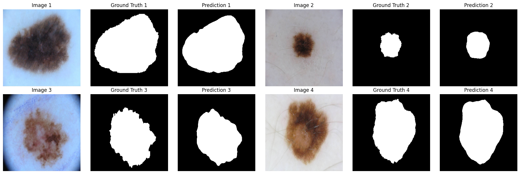
Results

On the test set, U-Net scored:

• Mean Dice Coefficient on Test Set: 0.6695
• Mean IoU on Test Set: 0.5642

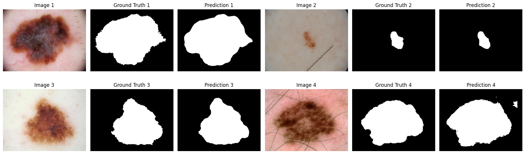
Four samples with their ground truth and U-Net prediction segmentation masks

The above metrics and qualitative comparison of image, ground truth segmentation, and predicted segmentation give a quantitative and qualitative measure of U-Net’s segmentation performance but understanding the model’s predictions and decision-making process requires squeezing some meaning out of model layers.

Grad-CAM and CAM Analysis

1. Grad-CAM (Bottleneck Layer):
   • Grad-CAM visualizes the focus of the bottleneck layer, which is responsible for encoding global context and structure.
   • The heatmap highlights the lesion’s edges and surrounding areas, suggesting that the model leverages boundary information to differentiate lesion from non-lesion regions.
2. CAM (Final Layer):
   • CAM visualizes the pixel-wise decision-making of the final layer, which produces the segmentation map.
   • The heatmap shows strong activation in regions corresponding to the lesion, with minimal attention to the surrounding healthy skin.

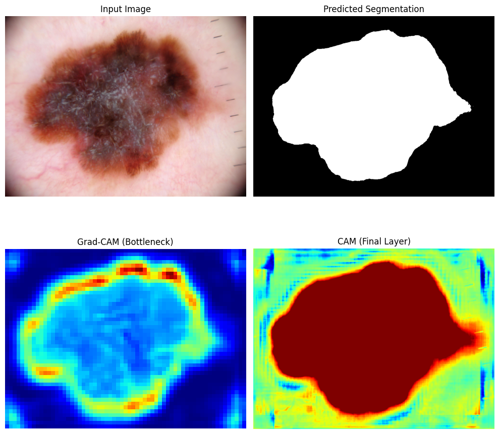
Input, predicted, CAM, and Grad-CAM visualization plot

It is hopefully clear why the U-Net structure is the way it is given the above plot.

• The bottleneck captures high-level semantic and structural information like the entire boundary around the lesion.
• The final layer refines predictions in order to get the dense pixel-level accuracy required for segmentation.

Discussion

While the IoU score seems low, its hard to see this lacking qualitatively. Below is an plot with U-Net’s segmentation of four input images. From a human perspective, the model appears to capture the essential features and boundaries effectively which is the main motivation behind medical image segmenation. Also here we can see U-Net’s IoU scores from the original paper from another segmentation competition on cell segmentation compared to 4 other methods:

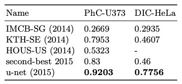
IoU scores of U-Net compared to other methods on a cell segmentation task [2].

For harder problems like in segmenting lesions rather than cells which are already fairly distinct from nearby structures, a score of 0.5642 is good.

Model 2: U-Net++

UNet++, an advanced extension of the UNet architecture, has proven effective in achieving high performance for medical segmentation tasks. This section delves into key innovations of UNet++, its training process, and showcases results through evaluation metrics and visualizations.

Architecture

UNet++ builds upon the standard UNet architecture by introducing nested dense skip connections and deep supervision. These enhancements address the inherent limitations of UNet, particularly the semantic gap between encoder and decoder features.

In the UNet architecture, the encoder extracts spatially fine-grained but semantically shallow features, while the decoder focuses on semantically rich but spatially coarse features. The direct fusion of these features via skip connections often results in a mismatch, leading to suboptimal performance. UNet++ tackles this issue by introducing intermediate dense convolutional blocks along the skip pathways, which progressively refine the encoder’s feature maps before merging them with the decoder.

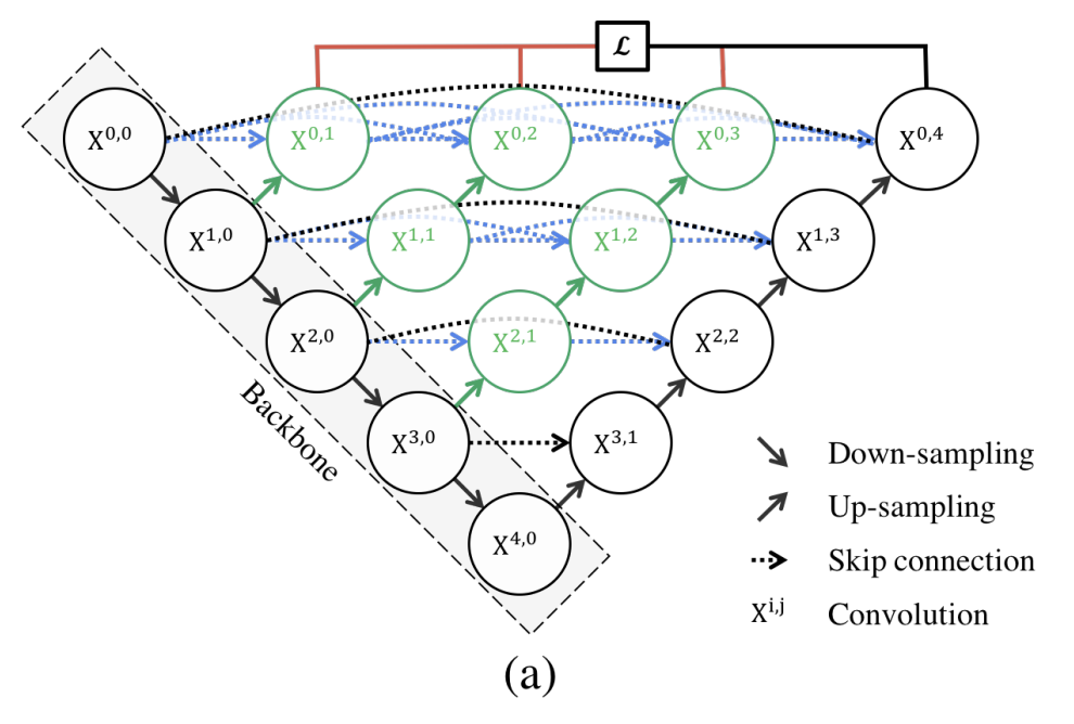
U-Net++ Architecture diagram from [3]

Key Features of UNet++

• Nested Dense Skip Connections: UNet++ replaces the plain skip connections of UNet with nested dense convolutional blocks. These blocks bridge the semantic gap between encoder and decoder feature maps by refining them through multiple convolutional layers. Each dense block combines outputs from earlier layers and upsampled features, ensuring better feature fusion.

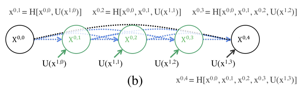
U-Net++ Architecture diagram from [3]

• Deep Supervision: UNet++ enables deep supervision by generating outputs at multiple levels of the decoder. This approach ensures better gradient flow during training and allows the model to operate in two modes during inference:
  • Accurate Mode: Combines outputs from all decoder levels for precise segmentation.
  • Fast Mode: Uses a single decoder level for quicker inference, trading off some accuracy for speed.

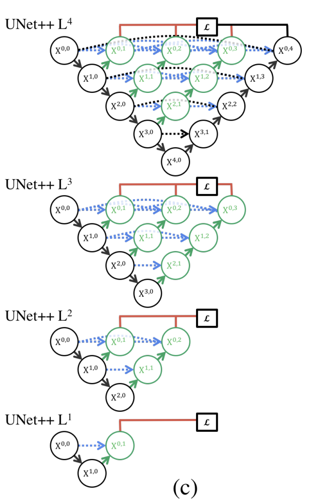
U-Net++ Training diagram from [3]

Code Implementation

Below is a basic implementation of the UNet++ architecture:

class VGGBlock(nn.Module):
    def __init__(self, in_channels, middle_channels, out_channels):
        super().__init__()
        self.relu = nn.ReLU(inplace=True)
        self.conv1 = nn.Conv2d(in_channels, middle_channels, 3, padding=1)
        self.bn1 = nn.BatchNorm2d(middle_channels)
        self.conv2 = nn.Conv2d(middle_channels, out_channels, 3, padding=1)
        self.bn2 = nn.BatchNorm2d(out_channels)

    def forward(self, x):
        out = self.conv1(x)
        out = self.bn1(out)
        out = self.relu(out)

        out = self.conv2(out)
        out = self.bn2(out)
        out = self.relu(out)

        return out

class NestedUNet(nn.Module):
    def __init__(self, num_classes, input_channels=3, deep_supervision=False, **kwargs):
        super().__init__()

        nb_filter = [32, 64, 128, 256, 512]

        self.deep_supervision = deep_supervision

        self.pool = nn.MaxPool2d(2, 2)
        self.up = nn.Upsample(scale_factor=2, mode='bilinear', align_corners=True)

        self.conv0_0 = VGGBlock(input_channels, nb_filter[0], nb_filter[0])
        self.conv1_0 = VGGBlock(nb_filter[0], nb_filter[1], nb_filter[1])
        self.conv2_0 = VGGBlock(nb_filter[1], nb_filter[2], nb_filter[2])
        self.conv3_0 = VGGBlock(nb_filter[2], nb_filter[3], nb_filter[3])
        self.conv4_0 = VGGBlock(nb_filter[3], nb_filter[4], nb_filter[4])

        self.conv0_1 = VGGBlock(nb_filter[0]+nb_filter[1], nb_filter[0], nb_filter[0])
        self.conv1_1 = VGGBlock(nb_filter[1]+nb_filter[2], nb_filter[1], nb_filter[1])
        self.conv2_1 = VGGBlock(nb_filter[2]+nb_filter[3], nb_filter[2], nb_filter[2])
        self.conv3_1 = VGGBlock(nb_filter[3]+nb_filter[4], nb_filter[3], nb_filter[3])

        self.conv0_2 = VGGBlock(nb_filter[0]*2+nb_filter[1], nb_filter[0], nb_filter[0])
        self.conv1_2 = VGGBlock(nb_filter[1]*2+nb_filter[2], nb_filter[1], nb_filter[1])
        self.conv2_2 = VGGBlock(nb_filter[2]*2+nb_filter[3], nb_filter[2], nb_filter[2])

        self.conv0_3 = VGGBlock(nb_filter[0]*3+nb_filter[1], nb_filter[0], nb_filter[0])
        self.conv1_3 = VGGBlock(nb_filter[1]*3+nb_filter[2], nb_filter[1], nb_filter[1])

        self.conv0_4 = VGGBlock(nb_filter[0]*4+nb_filter[1], nb_filter[0], nb_filter[0])

        if self.deep_supervision:
            self.final1 = nn.Conv2d(nb_filter[0], num_classes, kernel_size=1)
            self.final2 = nn.Conv2d(nb_filter[0], num_classes, kernel_size=1)
            self.final3 = nn.Conv2d(nb_filter[0], num_classes, kernel_size=1)
            self.final4 = nn.Conv2d(nb_filter[0], num_classes, kernel_size=1)
        else:
            self.final = nn.Conv2d(nb_filter[0], num_classes, kernel_size=1)


    def forward(self, input):
        x0_0 = self.conv0_0(input)
        x1_0 = self.conv1_0(self.pool(x0_0))
        x0_1 = self.conv0_1(torch.cat([x0_0, self.up(x1_0)], 1))

        x2_0 = self.conv2_0(self.pool(x1_0))
        x1_1 = self.conv1_1(torch.cat([x1_0, self.up(x2_0)], 1))
        x0_2 = self.conv0_2(torch.cat([x0_0, x0_1, self.up(x1_1)], 1))

        x3_0 = self.conv3_0(self.pool(x2_0))
        x2_1 = self.conv2_1(torch.cat([x2_0, self.up(x3_0)], 1))
        x1_2 = self.conv1_2(torch.cat([x1_0, x1_1, self.up(x2_1)], 1))
        x0_3 = self.conv0_3(torch.cat([x0_0, x0_1, x0_2, self.up(x1_2)], 1))

        x4_0 = self.conv4_0(self.pool(x3_0))
        x3_1 = self.conv3_1(torch.cat([x3_0, self.up(x4_0)], 1))
        x2_2 = self.conv2_2(torch.cat([x2_0, x2_1, self.up(x3_1)], 1))
        x1_3 = self.conv1_3(torch.cat([x1_0, x1_1, x1_2, self.up(x2_2)], 1))
        x0_4 = self.conv0_4(torch.cat([x0_0, x0_1, x0_2, x0_3, self.up(x1_3)], 1))

        if self.deep_supervision:
            output1 = self.final1(x0_1)
            output2 = self.final2(x0_2)
            output3 = self.final3(x0_3)
            output4 = self.final4(x0_4)
            return [output1, output2, output3, output4]

        else:
            output = self.final(x0_4)
            return output

Training

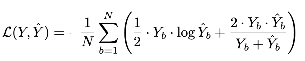
Training UNet++ involves carefully balancing the challenges of pixel-level accuracy and overall segmentation shape coherence. To achieve this, the training process leverages a combined loss function that integrates Binary Cross-Entropy (BCE) and Dice Loss. Let’s explore these components and their implementation in the training pipeline.

Combined Loss Function

The loss function used in UNet++ combines two key components:

1. Binary Cross-Entropy (BCE):
   • BCE ensures pixel-wise accuracy by penalizing incorrect predictions at the binary level.
   • It is particularly effective in handling class imbalances, where background pixels vastly outnumber foreground pixels.
2. Dice Loss:
   • Dice Loss focuses on maximizing the overlap between predicted segmentation masks and ground truth masks.
   • It ensures better shape preservation and structural accuracy in the segmentation output.

The combined loss is mathematically expressed as:

Code for Loss

Below is a code snippet illustrating the loss computation and training loop:

import torch
import torch.nn.functional as F
from torch.nn import Module

EPSILON = 1e-6

class DiceLoss(Module):
    def __init__(self):
        super().__init__()
    
    def forward(self, pred, mask):
        # Ensure size compatibility
        if pred.shape != mask.shape:
            raise ValueError(f"Shape mismatch: pred {pred.shape} vs mask {mask.shape}")
        # Flatten tensors for Dice computation
        pred = pred.flatten()
        mask = mask.flatten()
        # Compute intersection and Dice score
        intersect = (mask * pred).sum()
        dice_score = 2 * intersect / (pred.sum() + mask.sum() + EPSILON)
        dice_loss = 1 - dice_score
        return dice_loss

class CombinedLoss(Module):
    def __init__(self, weight_dice=0.2, weight_bce=0.8):
        super().__init__()
        self.weight_dice = weight_dice
        self.weight_bce = weight_bce
        self.dice_loss = DiceLoss()
        self.bce_loss = torch.nn.BCEWithLogitsLoss()
    
    def forward(self, pred, mask):
        # Ensure the predicted and target sizes are compatible
        if pred.shape[1:] != mask.shape[1:]:
            raise ValueError(f"Shape mismatch: pred {pred.shape} vs mask {mask.shape}")
        
        if pred.shape[1] == 1 and mask.dim() == 3:  # Handle (B, H, W) vs (B, C, H, W)
            mask = mask.unsqueeze(1)
        
        dice = self.dice_loss(torch.sigmoid(pred), mask) # Dice loss
        bce = self.bce_loss(pred, mask)         # BCEWithLogitsLoss
        combined_loss = self.weight_dice * dice + self.weight_bce * bce         # Weighted sum of Dice and BCEWithLogitsLoss
        return combined_loss

# Example usage
criterion = CombinedLoss(weight_dice=0.2, weight_bce=0.8)

The training process for UNet++ involves iterating over batches of input images and segmentation masks, computing the combined loss, and updating the model parameters using backpropagation. Below is the PyTorch-based training loop:

for epoch in range(EPOCHS):
    model.train()
    epoch_loss = 0.0

    with tqdm(total=len(dataloader), desc=f'Epoch {epoch+1}/{EPOCHS}', position=0, leave=True) as pbar:
        for step, (images, masks) in enumerate(dataloader):
            images = images.to(device)
            masks = masks.to(device)

            optimizer.zero_grad()
            predictions = model(images)

            loss = criterion(predictions, masks)
            loss.backward()
            optimizer.step()

            epoch_loss += loss.item()
            # Update progress bar
            pbar.update(1)
            pbar.set_postfix(loss=loss.item())

    avg_loss = epoch_loss / len(dataloader)
    print(f"Epoch {epoch+1} Average Loss: {avg_loss:.4f}")

Advantages of Combined Loss

By integrating BCE and Dice Loss, the training process ensures:

• Pixel-Level Accuracy: BCE Loss handles small-scale details effectively.
• Shape and Structure Preservation: Dice Loss maintains the overall consistency of segmentation masks.
• This combination proves to be highly effective for medical segmentation tasks, particularly in handling complex structures and class imbalances

Results

Evaluation Metrics

The performance of the UNet++ model was evaluated using two key metrics: the Mean Dice Coefficient and the Mean Intersection over Union (IoU). These metrics measure the overlap between the predicted segmentation masks and the ground truth masks.

1. Dice Coefficient (DSC): Measures the overlap between predicted and ground truth masks. A higher value indicates better segmentation.
2. Intersection over Union (IoU): Computes the ratio of the intersection and union of predicted and ground truth masks.

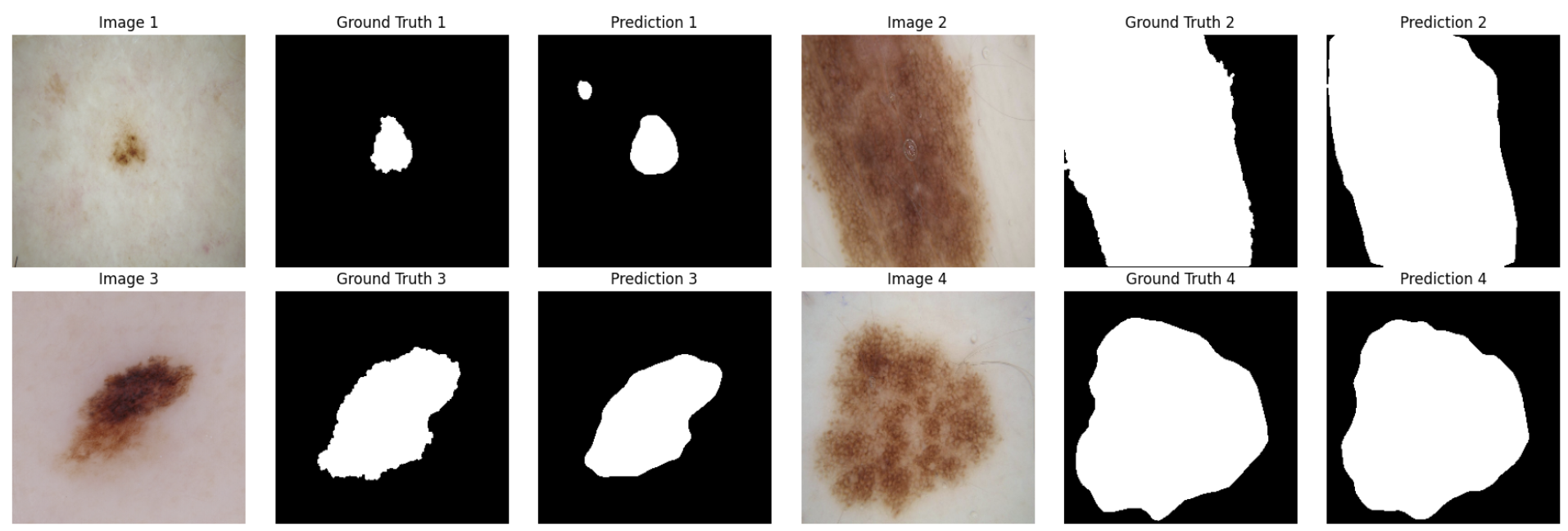
On the test set, U-Net++ scored:

• Mean Dice Coefficient on Test Set: 0.7839
• Mean IoU on Test Set: 0.6854

Prediction

Discussion

UNet++ demonstrates significant improvements over traditional UNet for medical segmentation tasks, owing to its architectural innovations and advanced training strategies. With its ability to generate accurate and reliable segmentations, it shows significant improvement from UNet in IoU score from 0.5642 to 0.6854 and 0.6695 to 0.7839 for DICE score. Also the predictions as shown above are slightly more fine grained and precise than U-Net, which is a reflection of the architectural improvements from U-Net to U-Net++.

Model 3: PSPNet

Semantic segmentation plays a critical role in computer vision and medical imaging by enabling precise delineation of regions of interest at the pixel level. Traditional segmentation approaches often struggle with capturing contextual information at multiple scales, which is crucial for accurately segmenting objects of varying sizes and shapes. In their paper Pyramid Scene Parsing Network [4], Zhao et al. proposed PSPNet, a deep learning model designed to enhance global context understanding by incorporating a Pyramid Pooling Module (PPM). This architecture was initially developed for scene parsing tasks but has shown great promise in medical image segmentation applications.

Architecture

PSPNet builds upon a pre-trained deep convolutional neural network (e.g., ResNet) as its backbone to extract high-level features. The unique contribution of PSPNet lies in its Pyramid Pooling Module (PPM), which efficiently aggregates multi-scale contextual information. The architecture consists of the following components:

• Backbone Network:
  • PSPNet utilizes a standard CNN backbone (e.g., ResNet-50 or ResNet-101) to produce intermediate feature maps at reduced spatial dimensions, capturing essential semantic information.
• Pyramid Pooling Module (PPM):
  • The PPM pools features at multiple scales (e.g., 1×1, 2×2, 3×3, and 6×6 grid regions) to capture spatial context at different levels.
  • The pooled features are upsampled to match the original feature map size.
  • All pooled features are concatenated with the original feature map to produce a multi-scale representation.
• Decoder and Output:
  • A 1×1 convolution layer reduces the dimensionality of the concatenated features.
  • A final softmax layer outputs pixel-wise class probabilities for segmentation.
• Auxiliary Loss (Optional):
  • To improve training stability, an auxiliary loss function is applied to intermediate features extracted from the backbone.

Overall, the model minimizes a pixel-wise cross-entropy loss, with auxiliary supervision optionally added to aid convergence.

Code Implementation

class PyramidPoolingModule(nn.Module):
    def __init__(self, in_channels, pool_sizes):
        super(PyramidPoolingModule, self).__init__()
        self.pool_sizes = pool_sizes
        self.stages = nn.ModuleList([
            nn.Sequential(
                nn.AdaptiveAvgPool2d(output_size),
                nn.Conv2d(in_channels, in_channels // len(pool_sizes), kernel_size=1, bias=False),
                nn.BatchNorm2d(in_channels // len(pool_sizes)),
                nn.ReLU(inplace=True)
            ) for output_size in pool_sizes
        ])
        self.bottleneck = nn.Sequential(
            nn.Conv2d(in_channels + in_channels // len(pool_sizes) * len(pool_sizes), in_channels, kernel_size=1, bias=False),
            nn.BatchNorm2d(in_channels),
            nn.ReLU(inplace=True)
        )

    def forward(self, x):
        h, w = x.size(2), x.size(3)
        pyramids = [x] + [F.interpolate(stage(x), size=(h, w), mode='bilinear', align_corners=False) for stage in self.stages]
        output = torch.cat(pyramids, dim=1)
        return self.bottleneck(output)

class PSPNet(nn.Module):
    def __init__(self, num_classes, backbone_features=512, pool_sizes=[1, 2, 3, 6]):
        super(PSPNet, self).__init__()
        self.encoder = nn.Sequential(
            nn.Conv2d(3, backbone_features // 2, kernel_size=3, stride=2, padding=1, bias=False),
            nn.BatchNorm2d(backbone_features // 2),
            nn.ReLU(inplace=True),
            nn.Conv2d(backbone_features // 2, backbone_features, kernel_size=3, stride=2, padding=1, bias=False),
            nn.BatchNorm2d(backbone_features),
            nn.ReLU(inplace=True)
        )

        self.pyramid_pooling = PyramidPoolingModule(backbone_features, pool_sizes)

        self.decoder = nn.Sequential(
            nn.Conv2d(backbone_features, 256, kernel_size=3, padding=1, bias=False),
            nn.BatchNorm2d(256),
            nn.ReLU(inplace=True),
            nn.Conv2d(256, num_classes, kernel_size=1)
        )

    def forward(self, x):
        h, w = x.size(2), x.size(3)
        x = self.encoder(x)
        x = self.pyramid_pooling(x)
        x = self.decoder(x)
        x = F.interpolate(x, size=(h, w), mode='bilinear', align_corners=False)  # Upsample to original size
        return x

Training

The PSPNet was trained on a training portion of the ISIC 2017 dataset contianing 2000 images and ground truth masks. We had the following hyperparameters for training:

• Image Dimensions: Height = 767, Width = 1022 (dataset images were this size)
• Batch Size: 4
• Learning Rate: 1e-3
• Optimizer: Adam
• Loss Function: Binary Cross Entropy with Logits (BCEWithLogitsLoss)
• Number of Epochs: 20
• In-channels/Out-channels: 3/1

Results

On the test set, PSPNet scored:

• Mean Dice Coefficient on Test Set: 0.6857
• Mean IoU on Test Set: 0.5857

Prediction

Discussion

PSPNet demonstrates a solid performance in medical image segmentation, thanks to its innovative Pyramid Pooling Module (PPM) that aggregates multi-scale contextual information. The ability to capture global context is particularly beneficial in medical imaging, where lesions, abnormalities, and anatomical features often vary significantly in size, shape, and appearance.

The model’s test set results, with a Mean Dice Coefficient of 0.6857 and a Mean IoU of 0.5857, highlight its effectiveness compared to baseline methods but also reveal some limitations relative to UNet++. While PSPNet outperforms the original UNet, it does not quite achieve the fine-grained accuracy of UNet++, as seen in the slightly lower Dice and IoU scores.

From a qualitative perspective, PSPNet’s predictions are robust in delineating boundaries and capturing essential features, particularly for lesions with relatively distinct edges. However, a potential drawback is its computational complexity, stemming from the multi-scale pooling operations and the use of high-capacity backbone networks like ResNet.

Conclusion

All three models showed promising results at segmenting skin lesions, with U-Net++ being the best of the three. All three exhibited adequate IoU and DICE scores, especially conisdering training was only done for 20 epochs on each model. If run for more epochs, we expect that these models would approach similar IoU results to the model papers cited, making them much more viable in real world scenarios.

Qualitatively looking at the results of segmenting lesions, it is clear that the essential features and boundaries are clearly defined by these models, albeit not perfectly. Despite this flaw, the promise of using semantic segmentation in the medical field seems clear. A doctor could benefit from getting a second opinion from a model trained on 100x more images than most doctors will see in their lifetime, as these models are able to pick up complicated features quicker than humans can.

Currently, medical semantic segmentation and other deep learning approaches for tackling complex medical tasks are not widespread. One reason is the regulatory aspect, as it is difficult to verify that these models are safe enough to use for clinical decision support. The other more limiting reason is the lack of large generalizable datasets. Patients have unique coniditons and journeys, and their data is difficult to generate synthetically. Even if this data was able to be generated synthetically, some deep learning approaches run into walls when applying models trained on synthetic data, and eventually the need for generalizable real world data becomes unavoidable.

As deep learning models become more sophisticated and entrenched in tasks, models such as the ones discussed in this paper will become much more relevant and widespread, easing clinical research and clinical decision support.

Reference

[1] Codella N, Gutman D, Celebi ME, Helba B, Marchetti MA, Dusza S, Kalloo A, Liopyris K, Mishra N, Kittler H, Halpern A. “Skin Lesion Analysis Toward Melanoma Detection: A Challenge at the 2017 International Symposium on Biomedical Imaging (ISBI), Hosted by the International Skin Imaging Collaboration (ISIC)”. arXiv: 1710.05006

[2] Ronneberger O, Fischer P, Brox T. “U-Net: Convolutional Networks for Biomedical Image Segmentation”. arXiv: 1505.04597.

[3] Z. Zhou, M. M. R. Siddiquee, N. Tajbakhsh, and J. Liang, “UNet++: A nested U-Net architecture for medical image segmentation,” in Proc. Int. Workshop Deep Learn. Med. Image Anal. Multimodal Learn. Clin. Decis. Support, 2018, pp. 3–11.

[4] Hengshuang Zhao, Jianping Shi, Xiaojuan Qi, Xiaogang Wang, Jiaya Jia. “Pyramid Scene Parking Network”. arXiv:1612.01105