3D Semantic Segmentation
3D semantic segmentation is a cornerstone of modern computer vision, enabling understanding of our physical world for applications ranging from embodied intelligence and robotics to autonomous driving. In 3D semantic segmentation, our goal is to assign a semantic label to every point in a LiDAR point cloud. Compared to pixel grids of 2D images, data from 3D sensors are complex, irregular, and sparse, lacking the niceties and biases in data we often exploit in processing 2D images. We will discuss 3 deep learning based approaches pioneering the field, namely PointNet, PointTransformerV3, and Panoptic-Polarnet.
Introduction
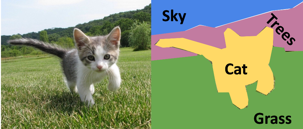
Fig 1. Example of 2D Semantic Segmentation [1].
Semantic segmentation is the backbone of many understanding tasks, from robotics to medical autonomy. 2D semantic segmentation involves assigning a class label to every pixel in an image. In 3D sematic segmentation, we extend this to assigning a class label to every point in a LiDAR point cloud. This is a much more challenging task due to the sparsity and unordered nature of point clouds, removing the helpful spatial locality and inherent density of 2D images we relied on to utilize traditional grid-based operations efficiency. Because of a lack of inherent spatial relationship between an unordered point set, we can’t naively process them through techniques like convolutions or patching. We discuss 3 deep learning based approaches to this challenge.
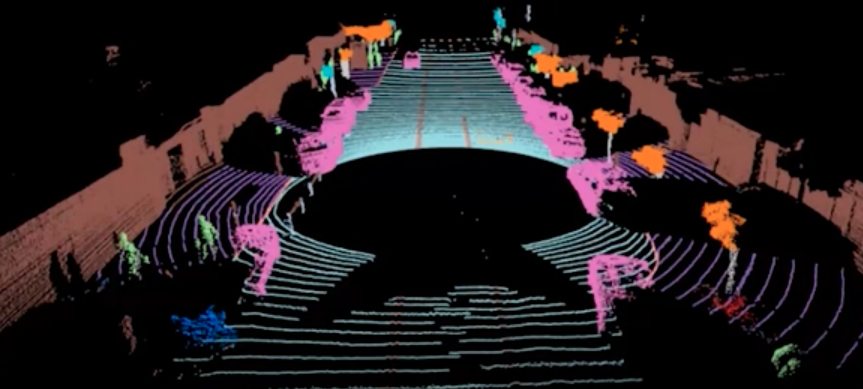
Fig 2. Example of 3D Semantic Segmentation [2].
3D Scene Representations
Point Clouds
We often represent 3D scenes as point clouds. A point cloud is a collection of \(n\) unordered points in 3D space:
\[\mathcal{P}=\{(x_i, y_i, z_i, f_i) : i=1,\ldots,n\}\]where each point is associated with a spatial location and \(k\)-dimensional \(f_i\) vector encoding optional features like color and intensity. Typically, we represent this as a matrix \(\mathbf{P}\in\mathbb{R}^{n\times (3+k)}\).
Point clouds are often collected from LiDAR sensors, which use the time of flight to obtain the 3D shape of a surrounding environment. LiDAR sensors shoot out impulses (via a packet of photons aka rays) to a scene, each of which bounce off an object \(z\) meters away. Given the time to return \(t_d\) and the speed of light, we can calculate
\[z=c\times t_d\times 0.5\]to get the distance each ray traveled before bouncing back. Combined with the ray angle data, we can capture a point cloud of the surface observed.
Voxel Grids
Voxels are the most natural extension of pixels into the 3-dimensional case, as they’re essentially 3D pixels. A voxel is a volumetric representation dividing a space into uniform cubes, represented as a 4-dimensional tensor containing information about each \((x,y,z)\) location in a scene:
\[\mathbf{V}\in\mathbb{R}^{X\times Y\times Z\times C}\]where each channel might contain RGB data, reflectance, and instance-level data like semantic labels.
Voxel size determines the grid’s resolution, which can lead to a tradeoff between high resolution and the number of unused voxels. Given that we typically only care about a 2D manifold/surface within the 3D space, voxels will capture mostly empty cubes, which can naturally lead to challenges with naively applying traditional operations like convolution. For this reason, we often work with binary voxels, tensors containing \(1\)’s for occupied space and \(0\)’s for empty space. Despite the benefit of spatial ordering that voxels give us, they suffer from a significant computational overhead to process.
Meshes
Meshes represent 3D objects as a collection of vertices, edges, and faces. This better aligns with the features we wish to learn from in 3D space, as they contain rich geometric and topological information. However, they’re irregular and more difficult to represent in a neural network, leading to extra complexity in processing and reconstruction.
Depth Images and BEV
Depth images and approaches like Bird’s Eye View fusion are approaches that project 3D data into 2D formats for computational simplicity. They often work alongside LiDAR-caera fusion for planning tasks.
Datasets and Evaluation Metrics
Datasets
The Stanford Large-Scale 3D Indoor Spaces (S3DIS) datset contains 3D point clouds of indoor environments like offices and conference rooms. The dataset contains 6 large-scale with 271 rooms. There are 13 semantic classes to learn from.
nuScenes is a large-scale autonomous driving dataset, containing 1000 scenes that each last 20 seconds. nuScenes is collected using a full sensor suite of LiDAR, radar, gamera, GPS, and IMU, lending itself well to a variety of self-driving tasks and settings. Semantic and instance segmentation labels are provided.
The Waymo Open Dataset is another large-scale autonomous driving dataset, containing LiDAR and camera data with 3D semantic labels. SemanticKITTI is another dataset that focuses on semantic and instance segmentation for urban street scenes.
Evaluation Metrics
As in 2D semantic segmentation, we’re primarily concerned with the Intersection over Union (IoU) score of our models. This measures the overall overlap between the predicted segmentation and the ground truth segmentation for each class. For a scene and class, we can calculate:
\[\text{IoU}=\frac{\mid\text{Predicted}\cap\text{Ground Truth}\mid}{\mid\text{Predicted}\cup\text{Ground Truth}\mid}\]Our goal is to minimize mIoU, the mean IoU over all classes.
Traditional Approaches
Early methods often drew heavily from 2D segmentation solutions, converting point clouds into voxel grids and applying 3D convolutional neural networks. However, voxelization has a drawback of high memory consumption and computational inefficiency, even when sparse methods were introduced, in comparison to point cloud-based methods. Multi-view approaches relying on systems like BEVFusion also focused on projecting 3D data into multiple 2D views for easier processing by relying on our existing 2D segmentation systems, but this also comes at a loss of spatial information due to projection.
For this reason, we’ll primarily explore solutions that operate directly on point clouds, which are more spatially efficient.
Deep Learning Approaches
PointNet
PointNet [2] was one of the first deep learning solutions to directly process raw point clouds without requiring a voxelization or projection step into a more structured input. It addressed three key challenges:
- Permutation invariance: point cloud data is inherently unordered and should handle all \(N!\) possible permutations of the input exactly the same.
- Interaction among points: in acknolwedging permutation invariance and foregoing a direct 3-dimensional structural representation, we should still account for the distance between points to maintain spatial information, much like in CNNs where local features aggregate and build up to more complex, semantic features.
- Transformation invariance: a geometric object’s representations and downstream predictions should ideally be identical under transformations like rotations.
In addressing these, PointNet became the new state-of-the-art as a backbone for 3D recognitions tasks, ranging from classification to part and instance segmentation, showing better robustness to rigid motions and perturbations.
The key to PointNets lie in finding an informative symmetic function. A symmetric function \(g\) is one that approximates a set on a function \(f\) as: \(f(\{x_1, \dots, x_n\}) \approx g(h(x_1), \dots, h(x_n)),\)
where \(f : 2^{\mathbb{R}^N} \to \mathbb{R}\) is the module we develop, \(h : \mathbb{R}^N \to \mathbb{R}^K\) is a transformation we’re learning (to extract features from the data), and
\(\gamma : \underbrace{\mathbb{R}^K \times \cdots \times \mathbb{R}^K}_{n} \to \mathbb{R}\) is a symmetric function we wrap these transformed outputs in to get a permutation invariant output. Instead, we can simply use an elementwise maximum function:
This is both very computationally efficient and empirically powerful. Intuitively, it tries captures the most important signals. \(\gamma\) and \(h\) are typically MLP networks to enable universal set function approximation, as we describe below.
PointNet also captures both global and local features for segmentation. It learns both a \(1024\)-dimensional global feature vector \(F\) and \(64\)-dimensional pointwise feature vectors \(f_i\), which are concatenated together before being passed into our segmentation head. This can improve performance on dense prediction tasks that rely on local features for final predictions.
Lastly, to address transformation invariance, one simply solution would be to just align an input set to a known orientation before feature extraction. This can be learned as an affine transformation, learned by a “T-net”, a smaller submdoule that’s a neural network on its own. This network’s architecture is similar to the overall network ifself, learning an affine transformation matrix \(A\) for canonicalizing input point clouds. We also use \(\ell_2\) regularization to keep the matrix orthogonal, which can prevent compressing space and losing information.
\[\ell=\lVert I-AA^T\rVert_F^2\]This empirically stabilized the training trajectory and convergence speed.
The authors of the PointNet paper also showed that PointNet maintained the universal approximation property–it can approximate any continuous set function on point clouds. Intuitively, we can interpret the model to show that it learns by summarizing shapes with a skeleton, a sparse subset of informative points. This guides the model to select interesting and informative points, regardless of their exact positions in 3D space, ane encode its reason for selecting them as a backbone. This improves robustness by only relying on a finite set of critical points per object, since as long as these critical points are unchanged the model is robust to other noise and occlusion.
PointNet scales linearly at $O(n)$ compute with respect to the number of points, while 3D convolutions would scale at $O(n^3)$!
PointNet++
While PointNet revolutioned deep learning in 3D at scale, it is not without its limitations. Particularly, it naively relies solely on MLP layers, lacking the locality and hierarchical feature extraction that made CNNs effective in both 2D and 3D cases, even if inefficient. PointNet is also unable to handle non-uniform LiDAR scans, as it assumes that its points are uniformly distributed. However, this is rarely true as real world point cloud have varying densities. For example, an autonomous vehicle will have greatly increased densities of nearby objects like pedestrians and street signs, but a low point density on distant roads, posing a challenge for PointNet to understand the environment’s structure.
PointNet++ [3] addresses these challenges by introducing hierarchical learning in three layers:
- First, a sampling layer uses farthest point sampling to select representative centroids for local regions. FPS chooses a subset \(\{x_1{i_1},x_{i_2},\ldots,x_{i_m}\}\) such that \(x_{i_j}\) is the most distant point from the the points \(\{x_1{i_1},x_{i_2},\ldots,x_{i_{j-1}}\}\) with respect to the rest of the points.
- Second, a grouping layer construct \(N'\times K\times (d+C)\) local regions around the \(N'\) \(d\)-dimensional centroids from an \(N\times (d+C)\) point set, where \(K\) is the number of neighbors to group together. This is done either via k-nearest neighbors selection, or a ball query where all points within a radius to a query point are added to a subgroup.
- A local mini-PointNet is applied to each region to extract features. Local geometry is encoded via relative coordinates.
This transforms the problem into smaller, more uniformly distributed sections that PointNet can handle, to be much more robust under non-uniform samling density. Similar to the inductive bias of CNNs, PointNet++ learns features at multiple set abstraction levels, where the above process is repeated many times to produce sets of fewer elements. This enables the model to learn fine-grained features and capture local geometry, but also provide contextual information via pooling layers.
Additionally, to handle the non-uniform sampling sampling inherent to point cloud data, PointNet++ introduces two new density adaptive layers. The first, Multi-Scale Grouping, uses a random dropout with a random rate of \(\theta\sim U(0, p)\) for \(o\leq 1\) on inputs to enforce training on data of various sparsities and various uniformities. This essentially extends on traditional neural network dropout by learning levels of sparsity, maintaining the same benefits like partially disentangling neurons. As this method is computationally expensive, since it would require running an entire PointNet forward pass even for very small centroids regions, PointNet++ also introduces Multi-resolution grouping, which essentially joins features from low density regions in a weighted manner.
Finally, they propose point feature propagation, where point features are propagated back into the original point cloud via an inverse distance-weighted interpolation based on $k$ nearest neighbors, which are connected from the set abstraction back into point space with skip connections. Similar to ResNet residual connections, this helps the model make high-resolution predictions.
PointNet++ set a new state-of-the-art for semantic segmentation, object detection, and classification tasks in 3D, outperforming PointNet on small datasets like ScanNet and ModelNet40. By exploiting inherent hierarchies in data more efficiently than techniques like 3D convolutions or even sparse convolutions, PointNet++ addressed many of the original assumptions PointNet made about its data, improving robustness. However, its computational costs are still much higher.
PointTransformer V3
PointTransformer V3 is the current state-of-the-art for 3D segmentation tasks, holding the highest accuracy on benchmarks like SemanticKITTI and ScanNet as of today.
PointTransformer V1 [11] marked 3D’s “ViT moment,” tailoring the attention mechanism for point clouds. Unlike PointNet’s reliance on MLPs, PointTransformer uses attention to share rich local and global features through unstructed point clouds. However, its reliance on \(k\) nearest neighbors and pairwise computation as a whole rendered it difficult to scale.
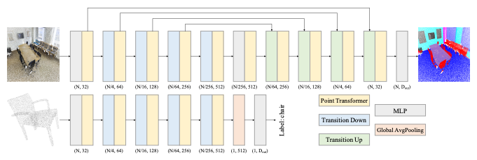
Fig 3. PointTransformer V1 Overview [11].
PointTransformer V2 [12] built on top of this by introducing Grouped Vector Attention (GVA) to enahnce computational efficiency. It presented a series of small optimizations on top of the original PointTransformer that added up, such as halving the total pairwise computations, increasing overall performance but reamining limited for large-scale dataset
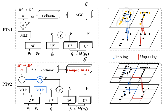
Fig 4. Comparison of PointTransformer V1 and PointTrasnformer V2 [12].
PointTransformer V3 (PTv3) [4] simplifies the architecture further and focuses on scale. One main focus of the project is point cloud serialization, a much more efficient method to transform unstructured point cloud data into a structured, serialized format for computation. This is done via space-filling curves, paths through a discrete high-dimensional space (like point space).
PTv3 focuses specifically on Z-order curves and Hilbert curves, both of which preserve spatial locality and improve computational efficiency by structuring data. They trasvers traverse 3D space through their specificied path, capturing discovered point clouds into a serialized 1D sequence. To leverage this locality preservations, the serlaization process assigns points basd on their position into a serialization code. This is similar to the embedding process for traditional transformers.
While original point transformers leveraged on neighborhood attention with neighborhood reduction stratgies relying heavily on pairwise computations, PTv3 intoduces patch attention as their attention mechanism, grouping points into non-overlapping patches and performing attention within each patch (similar to Swin Transformer). Models like PointNet++ also leveraged patch grouping strategies, but PTv3 leverages the inherent structure of the serialization for its patch grouping.
PTv3 incorporates these choices in a traditional U-Net like encoder-decoder structure for hierarchical feature analysis. It startrs by initializing serializations and embeddings from point cloud data. Then, the 4-stage encoder and decoder consists of several traditional transformer blocks with positional encoding, LayerNorm, Attention, and MLP layers. Although this method does approximate less optimal solutions than a k nearest neighbors based grouping or different attention mechanism, our formulation can now leverage traditional tooling for serialization and attention, helping the model scale easier. For example, the authors are able to scale up PTv3 to a larger receptive field of 4096 points while maintaing efficiency. The hypothesis that scale outweights intricate model design is validated in the results, as PointTransformer V3 sets a new SOTA on outdoor semantic segmentation tasks:
| Model | ScanNet200 Test | S3DIS 6-fold | nuScenes Test | Sem.KITTI Test | Waymo mIoU |
|---|---|---|---|---|---|
| PTv1 | - | 65.4 | 81.9 | 74.8 | - |
| PTv2 | 74.2 | 73.5 | 82.6 | 72.6 | 80.2 |
| PTv3 | 79.4 | 80.8 | 83.0 | 75.5 | 81.3 |
Table 1: Scores for PointTransformers on Semantic Segmentation tasks [7]
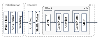
Fig 5. PointTrasnformer V3 Architecture [1].
PolarNet
Additionally, we discuss PolarNet [5], which utilizes 2D projections to handle point clouds.
It consists of 4 main steps: polar quantization, grid feature extraction, ring CNN, and projecting the prediction back to 3D.
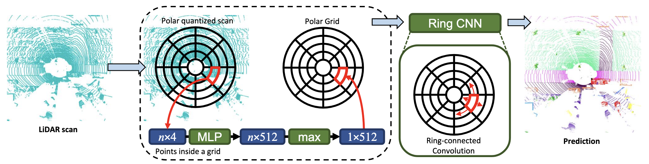
Fig 6. PolarNet Overview [5].
Polar Quantization
In order to tackle the challenges in dealing with 3D point clouds, PolarNet utilizes a 2D projection in order to make the data more manageable. It chooses to use a top-down projection, called a bird’s eye view (BEV). Using a BEV is especially well-suited for outdoor scenes, since objects do not typically overlap in the z-axis.
After projection, the points are grouped into a grid in order to utilize standard 2D CNN techniques. The main improvement in PolarNet stems from the method they use to convert points into a grid. Rather than using a traditional cartesian grid, they use polar coordinates. This helps tackle a major issue with cartesian grids: the fact that LiDAR point clouds tend to be much denser in areas closer to the center. By using polar, we more evenly distribute the number of points in each grid cell and minimize information loss due to quantization.
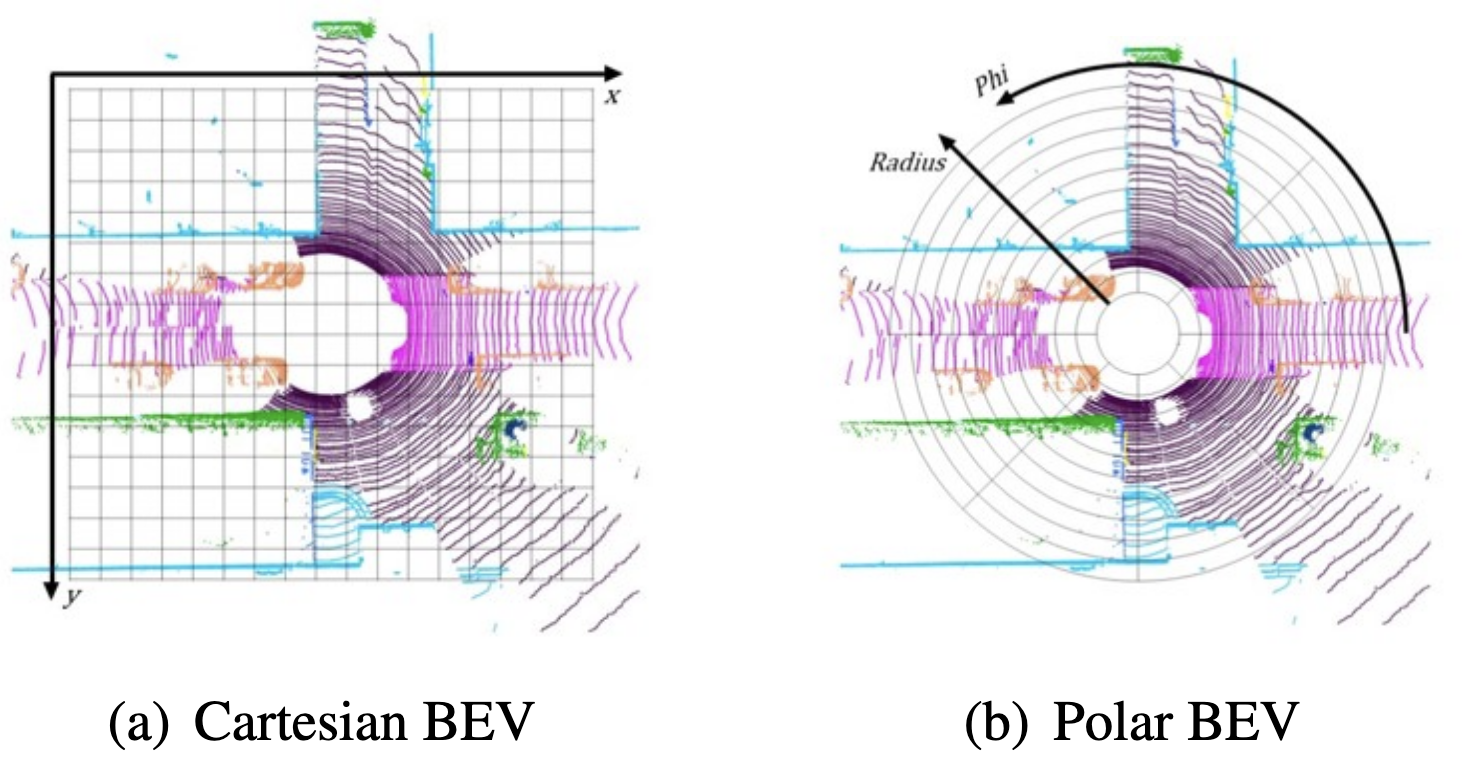
Fig 7. Comparison of Cartesian vs Polar BEV [5].
The authors use the SemanticKITTI dataset to perform several sanity checks:
-
Polar coordinates indeed help evenly spread out points, with each grid cell having \(0.7\pm 3.2\) points in cartesian BEV and \(0.7\pm 1.4\) points in polar BEV.
-
Assigning every point in each grid cell to its majority class results in high mIoU: \(97.3%\) for cartesian BEV and \(98.5%\) for polar BEV.
This suggests that using a BEV results in minimal information loss for outdoor scenes, and using the majority label for every point in a grid cell is a sound strategy for achieving high prediction scores.
Grid Feature Extraction
Now that we have grouped our points into grid cells, we want a fixed-length representation for each set of points.
We use a simplified PointNet model \(h(x)\) consisting of just an MLP. We apply \(h\) to each individual point in the grid cell, then apply a max-pooling operation for permutation invariance (since the point clouds are unordered).
Ring Convolution
After transforming the point cloud into a grid-based representation, we are almost ready to build a standard CNN model.
However, due to the geometry of polar coordinates, the angular edges of the matrix representing the grid are also spatially connected to each other (since \(0^\circ\) and \(359^\circ\) are next to each other). Thus, we must account for this when designing our convolutional layers.
Luckily, it is fairly easy to perform a ring convolution: one can simply pad the angular dimension of the matrix with a copy of itself. Making a copy of the original data and putting them side-by-side is a standard technique for designing cyclic algorithms.
PolarNet utilizes a standard UNet model with 4 encoding and 4 decoding layers, replacing the convolutional layers with ring convolutions.
Prediction
The output of the CNN predicts a class label for each grid cell. During training, the ground truth label for each grid cell is computed using majority vote, and mIoU is used as the loss function.
At test time, for each grid cell \(i\) with label \(c\), we assign every point that maps to cell \(i\) with the label \(c\).
This achieves fairly robust results without the need for developing any particularly novel architecture. Additionally, the resulting model is extremely lightweight and can be run in real-time applications.
Panoptic-PolarNet
The authors have also extended PolarNet for panoptic segmentation, for which we provide a brief summary. Panoptic segmentation aims to unify instance and semantic segmentation, assigning a class label to every point, and assigning instance IDs to points belonging to a “thing” class (e.g. car). For points belonging to a “stuff” class (e.g. sky), we do not assign an instance ID.
In Panoptic-PolarNet [6], additional prediction heads are added to the end of the UNet backbone. For each grid cell, a heatmap of likely object centers is generated. Grid cells with the same centers are grouped together, and a deterministic fusion step is used to combine the groupings with the semantic segmentation prediction to produce a panoptic segmentation prediction. A combined loss function is used to optimize all of the prediction heads simultaneously.
Panoptic quality is used as a metric to evaluate panoptic segmentation:
\[\text{PQ}=\text{SQ}\cdot \text{RQ}\]combining segmentation quality (IoU) with recognition quality (often F1 score, measuring precision and recall).
Panoptic-PolarNet achieved state of the art performance on SemanticKITTI panoptic segmentation when it was published.
Results
| test mIoU | Year | |
|---|---|---|
| PTv3 | 75.5% | 2023 |
| PolarNet | 57.2% | 2020 |
| PointNet++ | 20.1% | 2017 |
| PointNet | 14.6% | 2016 |
Table 2: Scores for SemanticKITTI 3D Semantic Segmentation task [7]
Comparisons
PointNet was the first model to process raw point cloud data without a spatial reconstruction, making way to a family of models that operate directly on unordered and unstructured point sets. It enabled linear time scaling of compute as opposed to cubic time scaling of 3D convolutions. By developing a permutation and transformation invariant model, and still relying on relatively simple MLPs, it reached a new state-of-the-art while still being the most efficient of its time. However, it lacked locality and hierarhical feature extraction, both of which are cornerstones of phyiscal data.
PointNet++ built atop these by leveraging PointNets in a hierarchical manner. By handling non-uniformly dense point clouds via density adaptive layers, it’s more robust to LiDAR samples seen in the wild. However, it’s still more computationally complex that PointNet and relatively low mIoU compared to moderl attention-based models.
The current state-of-the-art is PointTransformerV3, presented at CVPR 2024, which utilized point cloud serialization via space-filling curves to combine attention with a cheap spatial structuring of point set data. It also usees a relatively simple U-Net like transformer architecture, embracing ease of scaling over complexity.
PolarNet is an alternative lightweight architecture capable of real-time performance. It improves greatly on PointNet with a CNN, by utilizing a polar BEV projection, but falls behind PointTransformerV3 in terms of accuracy.
Running Pointnet++
We utilize the Pointnet++ Pytorch implementation [8] for semantic segmentation on the S3DIS indoor dataset.
The S3DIS dataset can be downloaded by filling out this form.
The repository supports running Pointnet and Pointnet++ for classification, part segmentation, and semantic segmentation and is implemented in Python with pytorch as its only dependency, making it easy to run in Colab. Our Colab notebook can be found here.
Minor modifications to the train and test scripts need to be made due to np.float being deprecated by Numpy. Additionally, the train and test scripts expect the dataset to be in different locations, so we create a symlink to account for this.
The model outputs visualizations as an OBJ file that we can compare to the ground truth in Meshlab, an open source visualization tool. We display one set of results from our model.
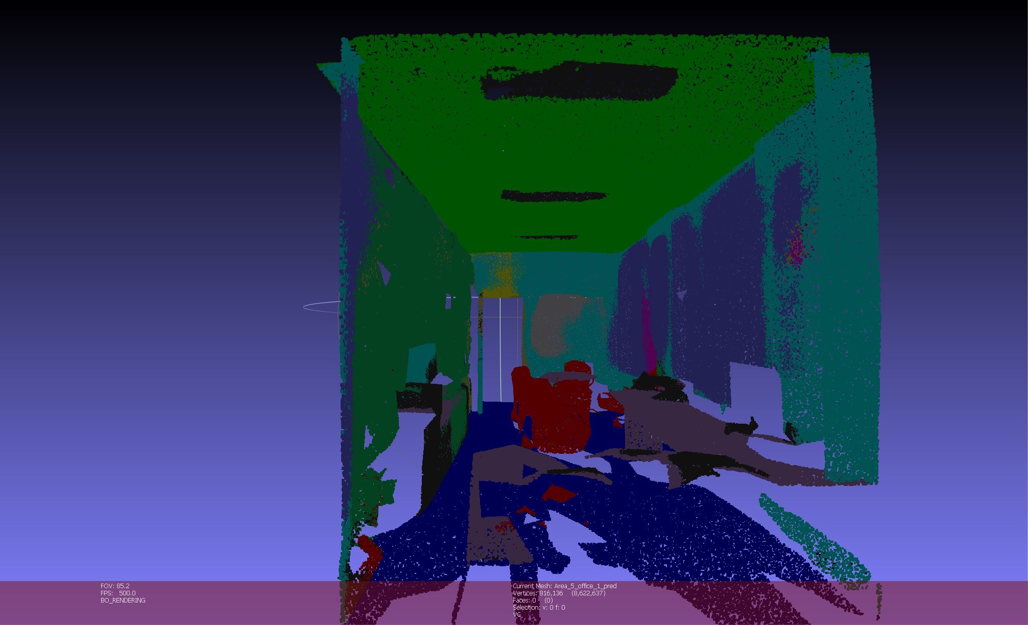
Fig 8. Prediction for an office scene
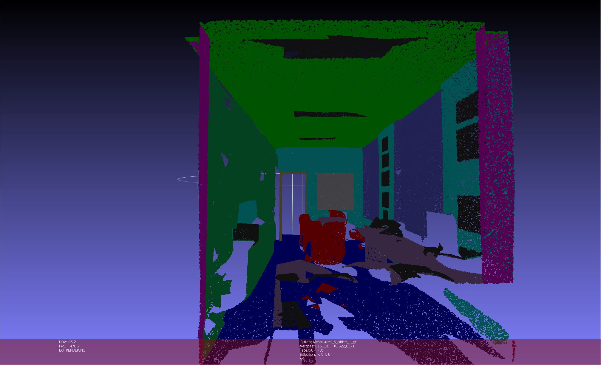
Fig 9. Ground truth for an office scene
S3DIS has 13 classes: ceiling, floor, wall, beam, column, window, door, table, chair, sofa, bookcase, board, and clutter.
The model achieves very high mIoU for ceilings and floors, but often confuses walls, windows and bookcases. For this office scene, Pointnet++ impressively detects the chairs and tables.
References
[1] Zhou, Bolei. Lecture 14: Detection + Segmentation. Computer Science 163: Deep Learning for Computer Vision, 18 Nov. 2024, University of California, Los Angeles. PowerPoint presentation.
[2] Waymo Open Dataset, 17 June 2024. CVPR Workshop on Autonomous Driving.
[2] Charles R Qi, Hao Su, Kaichun Mo, and Leonidas J Guibas. “Pointnet: Deep learning on point sets for 3d classification and segmentation.” CVPR. 2017.
[3] Charles R Qi, Li Yi, Hao Su, and Leonidas J Guibas. “Point-net++: Deep hierarchical feature learning on point sets in a metric space.” NeurIPS. 2017
[4] Wu, Xiaoyang, Li, Jiang, Peng-Shuai, Wang, Zhijian, Liu, Xihui, Liu, Yu, Qiao, Wanli, Ouyang, Tong, He, Hengshuang, Zhao. “Point Transformer V3: Simpler, Faster, Stronger.” CVPR. 2024.
[5] Yang Zhang, Zixiang Zhou, Philip David, Xiangyu Yue, Ze-rong Xi, Boqing Gong, and Hassan Foroosh. “Polarnet: An improved grid representation for online lidar point clouds se-mantic segmentation.” CVPR. 2020.
[6] Zhou, Zixiang, Yang, Zhang, Hassan, Foroosh. “Panoptic-PolarNet: Proposal-free LiDAR Point Cloud Panoptic Segmentation.” CVPR. 2021.
[7] “Papers with Code: 3D Semantic Segmentation on SemanticKITTI Leaderboard.” Papers with Code, 2024, https://paperswithcode.com/sota/3d-semantic-segmentation-on-semantickitti
[8] Xu Yan. “Pointnet/Pointnet++ Pytorch”. https://github.com/yanx27/Pointnet_Pointnet2_pytorch. 2019.
[10] O. Vinyals, S. Bengio, and M. Kudlur. “Order matters: Sequence to sequence for sets.” arXiv preprint arXiv:1511.06391, 2015.
[11] Hengshuang Zhao, Li Jiang, Jiaya Jia, Philip Torr, and Vladlen Koltun. Point Transformer. arXiv preprint arXiv:2012.09164, 2021. https://arxiv.org/abs/2012.09164
[12] Xiaoyang Wu, Yixing Lao, Li Jiang, Xihui Liu, and Hengshuang Zhao. Point Transformer V2: Grouped Vector Attention and Partition-based Pooling. arXiv preprint arXiv:2210.05666, 2022. https://arxiv.org/abs/2210.05666