On Exploring Modern Facial Recognition Models with Bounding Box Detection
This project explores the application of four modern object detection models—Faster R-CNN, SSD, YOLOv5, and EfficientDet—for facial recognition tasks. Each model was evaluated based on its performance, speed, and scalability using a curated dataset of face images. Faster R-CNN exhibited high accuracy, making it ideal for precision-focused tasks, but its slower inference speed limited real-time applicability. SSD offered a balanced trade-off between speed and accuracy, suitable for diverse scenarios. YOLOv5 excelled in real-time performance, demonstrating a strong balance of speed and precision. EfficientDet showcased scalability and multi-scale detection capabilities but faced limitations in computational efficiency for face-specific tasks. These evaluations highlight the trade-offs between accuracy, speed, and resource constraints, providing insights for model selection in real-world facial recognition applications.
- Introduction
- Dataset
- Preprocessing
- Explored Models
- Example Model Outputs
- Final Words & Conclusion
- Reference
Introduction
Facial recognition has become one of the most transformative technologies in computer vision, with applications spanning security, social media, healthcare, and beyond. This blog post explores the challenges and opportunities in implementing modern facial recognition systems, focusing on the evaluation of four prominent object detection models. By comparing Faster R-CNN, SSD, YOLOv5, and EfficientDet, we aim to highlight the trade-offs between accuracy, speed, and scalability, providing insights into model selection for real-world applications.
Dataset
For this project, we used a dataset sourced from Kaggle (link), specifically curated for face detection tasks. The dataset comprises \(16,700\) high-quality images focused exclusively on detecting human faces. These images were collected using the OIDv4 toolkit, a scraping tool for extracting data from Google Open Images. The dataset includes detailed annotations provided in two formats: the Label file and yolo_format_labels. The Label file contains bounding box coordinates in pixel values, while the yolo_format_labels employs the normalized YOLO format, where bounding box values are normalized to fall within a range of \(0\) to \(1\) relative to the image dimensions.
The dual-format annotation is particularly advantageous for deep learning applications, offering flexibility in adapting to different model architectures and scaling techniques. The annotations are structured as plain text files, with each line representing a bounding box in the following format: <class_id> <x_center> <y_center> <box_width> <box_height>. This format is efficient for training object detection models and adheres to conventions widely used in computer vision research.
Although the dataset is approximately \(5\) GB in size, we used a smaller subset for this project to ensure faster and more affordable training. Specifically, we utilized \(5,000\) images for the training phase. These images were carefully selected to preserve the diversity and quality of the larger dataset while maintaining computational feasibility. Each image has a corresponding annotation file containing the bounding boxes for all detected faces in the image.
Overall, the dataset’s high quality and focus on face detection make it highly suitable for developing and optimizing robust face detection models. By using a subset of this dataset, we aimed to strike a balance between computational efficiency and model performance, ensuring that the training and evaluation processes remained both effective and accessible.
The YOLO Convention
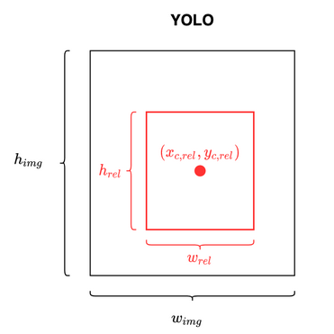
YOLO (You Only Look Once) adopts a specific convention for object detection tasks, which defines how objects are annotated and predictions are structured.
In this convention, each object in an image is represented by a bounding box defined by its center coordinates (\(x\), \(y\)), width (\(w\)), and height (\(h\)), normalized relative to the image’s dimensions. The associated class labels are encoded as integer indices corresponding to a predefined list of categories.
Preprocessing
The preprocessing step for this project was kept intentionally minimal to maintain simplicity and ensure a focus on the model’s performance. The data was handled as follows:
- Data Loading: The images were loaded using Python’s PIL (Pillow) library. This step ensured that all images were correctly read and handled in their original formats.
- Tensor Conversion: After loading, the images were converted to PyTorch tensors. This conversion facilitated their use as input for the PyTorch-based deep learning model.
No additional preprocessing steps, such as resizing, normalization, or augmentation, were performed during this stage.
Explored Models
In this project, we explored several object detection models, each offering distinct advantages tailored to specific needs. The models evaluated are Faster R-CNN, known for its high accuracy but slower inference speed; Single Shot Multibox Detector (SSD), which balances speed and accuracy; YOLOv5, optimized for real-time detection; and EfficientDet, valued for its scalability and efficiency. The following sections provide an in-depth look at each model.
Faster R-CNN
Overview
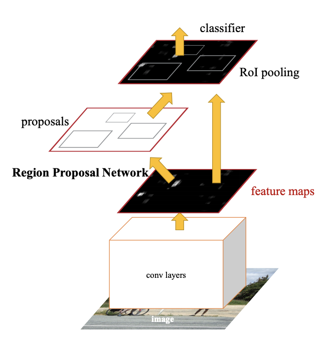
Faster R-CNN, or Faster Region-based Convolutional Neural Network, is a state-of-the-art deep learning model designed for object detection. Object detection involves identifying and localizing objects within an image, a fundamental challenge in computer vision. Faster R-CNN improves upon earlier models such as R-CNN and Fast R-CNN by introducing a significant innovation: the Region Proposal Network (RPN). By integrating the entire detection pipeline into a single framework and eliminating the need for external region proposal algorithms, Faster R-CNN achieves both high accuracy and significant computational efficiency.
Feature Extraction Backbone
The first component of Faster R-CNN is its feature extraction backbone, which is typically a Convolutional Neural Network (CNN) such as ResNet-50. The backbone processes the input image to generate feature maps, which are rich, compact representations of the image. These feature maps retain important spatial and contextual information necessary for detecting and classifying objects. The backbone essentially transforms the high-dimensional input image into a lower-dimensional but highly informative set of features, making it easier for subsequent components to operate effectively.
Region Proposal Network (RPN)
The Region Proposal Network (RPN) is a core innovation in Faster R-CNN and is responsible for generating candidate regions of interest (RoIs). These regions are the parts of the image likely to contain objects. The RPN operates by sliding small convolutional filters across the feature maps produced by the backbone. For each region it evaluates, the RPN predicts two outputs: objectness scores (to indicate whether the region contains an object) and bounding box coordinates (to suggest the location of the object).
To hypothesize object locations, the RPN uses anchor boxes, which are fixed-sized reference boxes of various shapes and sizes. After generating multiple proposals, the RPN applies a process called Non-Maximum Suppression (NMS) to filter out redundant or overlapping regions. This ensures that only the most relevant proposals are passed to the next stage for further analysis.
ROI Head
The final stage of Faster R-CNN is the ROI Head, which processes the regions proposed by the RPN to refine their predictions. Since the Regions of Interest (RoIs) vary in size, the ROI Head uses a technique called ROI Pooling or ROI Align to standardize them into fixed-size feature maps. These standardized features are passed through fully connected layers, which perform two key tasks. First, they classify the object within each RoI into specific categories or label it as background. Second, they adjust the bounding box coordinates to improve localization accuracy. This stage ensures that the final predictions are precise and well-aligned with the objects in the image.
Setup and Initialization
import torch
import torchvision
from torchvision.models.detection import fasterrcnn_resnet50_fpn
from torchvision.models.detection.faster_rcnn import FastRCNNPredictor

# Load a pre-trained Faster R-CNN model
model = fasterrcnn_resnet50_fpn(weights=torchvision.models.detection.FasterRCNN_ResNet50_FPN_Weights.DEFAULT)

# Modify the model for the specific dataset (single "face" class + background)
num_classes = 2  # 1 class (face) + background
in_features = model.roi_heads.box_predictor.cls_score.in_features  # Input features for the classifier
model.roi_heads.box_predictor = FastRCNNPredictor(in_features, num_classes)
Training and Optimization
import torch
import torch.optim as optim
from tqdm import tqdm

# Define the optimizer
optimizer = optim.SGD(model.parameters(), lr=0.005, momentum=0.9, weight_decay=0.0005)

# Learning rate scheduler
lr_scheduler = torch.optim.lr_scheduler.StepLR(optimizer, step_size=3, gamma=0.1)

# Training loop
num_epochs = 10  # Adjust as needed
device = torch.device("cuda") if torch.cuda.is_available() else torch.device("cpu")
model.to(device)

for epoch in range(num_epochs):
    model.train()
    epoch_loss = 0

    # Iterate through the data loader
    for images, targets in tqdm(train_loader):
        # Move data to the device
        images = [image.to(device) for image in images]
        targets = [{k: v.to(device) for k, v in target.items()} for target in targets]

        # Zero the parameter gradients
        optimizer.zero_grad()

        # Forward pass
        loss_dict = model(images, targets)
        losses = sum(loss for loss in loss_dict.values())

        # Backward pass and optimization
        losses.backward()
        optimizer.step()

        epoch_loss += losses.item()

    # Step the scheduler
    lr_scheduler.step()
Faster R-CNN is trained end-to-end, meaning all components—the feature extraction backbone, the RPN, and the ROI Head—are optimized simultaneously. This holistic approach eliminates the need for separate training steps or external proposal generation methods, making Faster R-CNN both efficient and streamlined. The training process involves optimizing two objectives: generating high-quality proposals through the RPN and ensuring accurate classification and localization through the ROI Head.
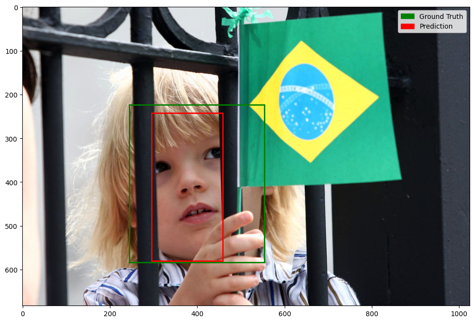
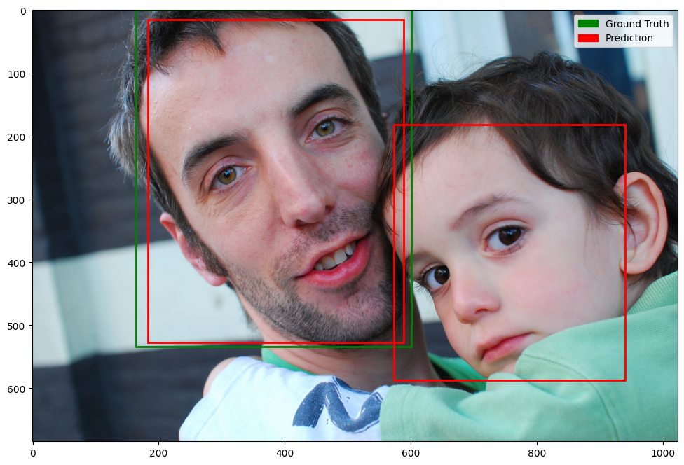
Observations
The evaluated IoU for the trained model was \(0.66\), indicating that the predicted bounding boxes, on average, overlapped significantly with the ground truth boxes. This value demonstrates the model’s capability to detect and localize faces effectively, though there is room for further improvement through additional fine-tuning, hyperparameter optimization, or enhancing the dataset.
Single Shot Multibox Detector (SSD)
Overview
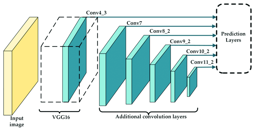
Single Shot Detector (SSD) models are popular in facial recognition systems due to their efficient single-pass architecture that processes images in real-time while maintaining reasonable accuracy. The model uses multiple convolutional layers at different scales to detect faces of varying sizes, making it effective for diverse scenarios. While SSD models excel in speed and computational efficiency, making them ideal for real-time applications like surveillance systems and mobile apps, they do have limitations - they may struggle with very small faces, extreme angles, poor lighting conditions, and partial occlusions, and generally offer lower accuracy compared to slower two-stage detectors like R-CNN variants. Despite these tradeoffs, their balanced combination of speed and accuracy makes them a practical choice for many commercial facial recognition applications where real-time processing is crucial.
Implementation
We implemented a Single Shot Detector (SSD) for face detection using a modified VGG-16 backbone network. The model was trained on a dataset of \(5000\) face images at \(640\times640\) resolution. Training was performed using the Adam optimizer with a learning rate of \(0.001\) and batch size of \(4\). The backbone network contains four convolutional blocks with increasing channel dimensions (\(64\rightarrow128\rightarrow256\rightarrow512\)), each followed by ReLU activation and MaxPooling (except the final block).
class SSDFaceDetector(nn.Module):
  def __init__(self):
    super(SSDFaceDetector, self).__init__()

    # Base network (VGG-16 like, simplified)
    self.features = nn.Sequential(
      nn.Conv2d(3, 64, kernel_size=3, padding=1),
      nn.ReLU(inplace=True),
      nn.MaxPool2d(kernel_size=2, stride=2),

      nn.Conv2d(64, 128, kernel_size=3, padding=1),
      nn.ReLU(inplace=True),
      nn.MaxPool2d(kernel_size=2, stride=2),

      nn.Conv2d(128, 256, kernel_size=3, padding=1),
      nn.ReLU(inplace=True),
      nn.MaxPool2d(kernel_size=2, stride=2),

      nn.Conv2d(256, 512, kernel_size=3, padding=1),
      nn.ReLU(inplace=True),
    )

    # Extra feature layers
    self.extra_features = nn.Sequential(
      nn.Conv2d(512, 256, kernel_size=1),
      nn.ReLU(inplace=True),
      nn.Conv2d(256, 512, kernel_size=3, padding=1, stride=2),
      nn.ReLU(inplace=True),
    )

    # Regression head for bounding box prediction
    self.loc = nn.Sequential(
      nn.Conv2d(512, 4, kernel_size=3, padding=1),  # 4 values for bbox (x, y, w, h)
    )

    # Classification head for face/no-face prediction
    self.conf = nn.Sequential(
      nn.Conv2d(512, 2, kernel_size=3, padding=1),  # 2 classes (face, background)
    )
Performance Results
The model achieved moderate performance with a validation accuracy of \(79\%\) and a mean IoU of \(0.65\). Training loss stabilized around \(1.45\), while validation loss settled at \(1.62\). Inference speeds of \(22\) FPS on GPU.
Hyperparameter Tuning
Through extensive experimentation, we identified optimal hyperparameter configurations for our face detection task. Learning rate proved to be the most critical parameter, with \(0.001\) providing the best balance between convergence speed and stability - higher values led to unstable training while lower values converged too slowly. The Adam optimizer outperformed both SGD and RMSprop, likely due to its adaptive learning rate mechanics. We found a batch size of \(4\) to be optimal given memory constraints and training dynamics, though larger batches might improve performance with sufficient computational resources. The loss function weighting between localization and classification (set to 1:1) proved effective, as increasing the weight of either component decreased overall performance. These settings resulted in stable training and the best overall performance metrics.
YOLOv5
Overview
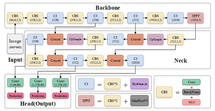
YOLOv5 (You Only Look Once version 5) is one of the most efficient and widely used object detection frameworks. It leverages cutting-edge deep learning techniques to balance speed, accuracy, and resource efficiency, making it a preferred choice for applications ranging from autonomous driving to medical image analysis. Unlike traditional two-stage detectors like Faster R-CNN, YOLOv5 performs object detection in a single pass, significantly reducing inference time while maintaining high detection accuracy.
Strengths of YOLOv5
-
Real-Time Processing: YOLOv5 excels at real-time object detection with minimal latency, making it ideal for applications requiring high-speed inference, such as traffic monitoring or robotics.
-
High Accuracy with Low Compute Requirements: Unlike other object detection frameworks, YOLOv5 achieves a strong balance between accuracy and efficiency, even on resource-constrained devices like edge devices and embedded systems.
-
Enhanced Data Augmentation: YOLOv5 employs advanced augmentation techniques like mosaic augmentation and mix-up, which improve the model’s robustness to variations in scale, lighting, and occlusions.
-
Flexibility Across Applications: YOLOv5 supports multiple configurations (e.g., YOLOv5s, YOLOv5m, YOLOv5l, and YOLOv5x), allowing users to trade off speed and accuracy based on application requirements.
Implementation
# Install YOLOv5 requirements
!pip install -U torch torchvision albumentations matplotlib opencv-python

# Clone YOLOv5 repository
!git clone https://github.com/ultralytics/yolov5
%cd yolov5
import torch
from yolov5.models.common import DetectMultiBackend
from yolov5.utils.dataloaders import create_dataloader
from yolov5.utils.general import check_img_size, non_max_suppression
from yolov5.utils.plots import Annotator, colors
from yolov5.utils.torch_utils import select_device

# Verify PyTorch installation and GPU availability
device = select_device('cuda:0')
# Training
!python train.py --img 5000 --batch 16 --epochs 10 --data "/content/drive/MyDrive/finalproj/data/data_updated.yaml" --weights yolov5s.pt --name facial_recognition

# Validation
!python val.py --weights runs/train/facial_recognition4/weights/best.pt --data "/content/drive/MyDrive/finalproj/data/data_updated.yaml" --img 640

# Detection
!python detect.py --weights runs/train/facial_recognition4/weights/best.pt --source "/content/drive/MyDrive/finalproj/data/images/val" --img 640
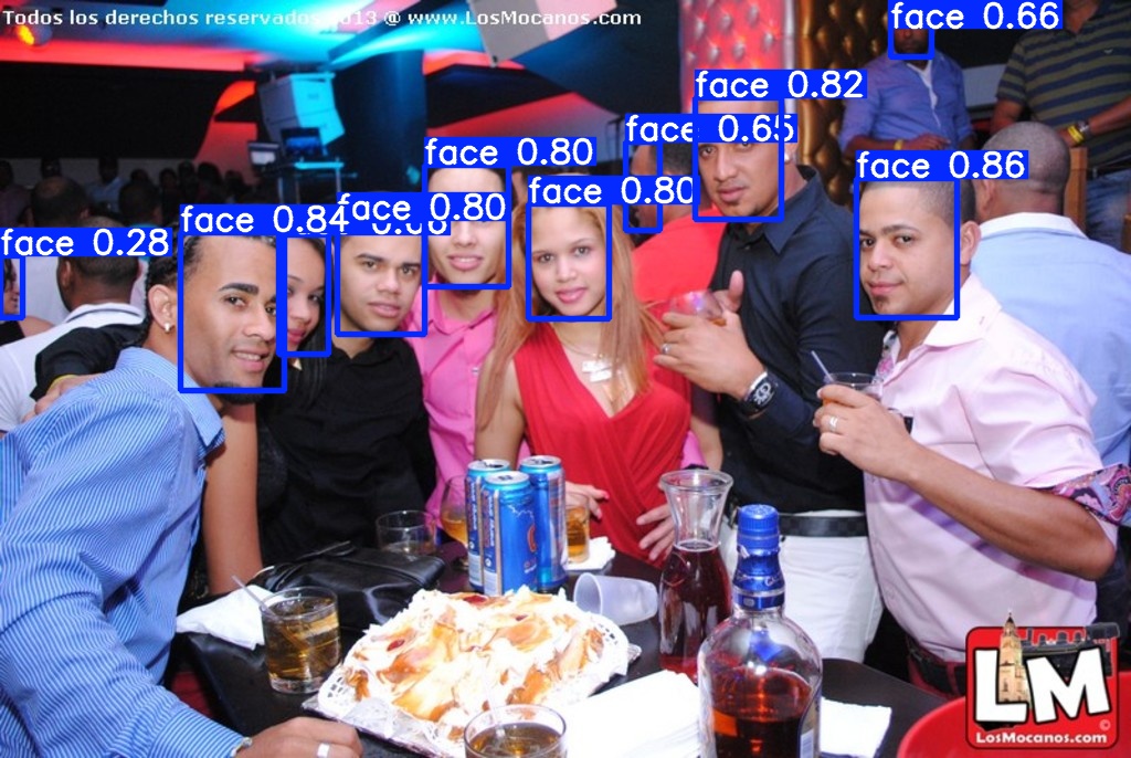
Observations
The high precision score of \(0.883\) indicates that YOLOv5 is highly effective at minimizing false positives, ensuring that most predicted bounding boxes are accurate. Meanwhile, the recall value of \(0.79\) suggests that a majority of the actual objects were identified, although there is room for improvement in reducing false negatives. The mAP50 score of \(0.86\) reflects strong performance at the IoU threshold of \(0.50\), showcasing the model’s ability to localize and classify objects accurately. However, the mAP50-95 score of \(0.548\) highlights a drop in performance under stricter IoU thresholds, pointing to potential limitations in precise localization, particularly for small or overlapping objects.
YOLOv5 has proven to be a highly effective object detection framework, balancing precision, recall, and computational efficiency. Its strengths lie in real-time performance and versatility across a wide range of applications. However, challenges with recall and precise localization under stricter IoU thresholds highlight areas for improvement, particularly in tasks requiring higher granularity.
EfficientDet
Overview
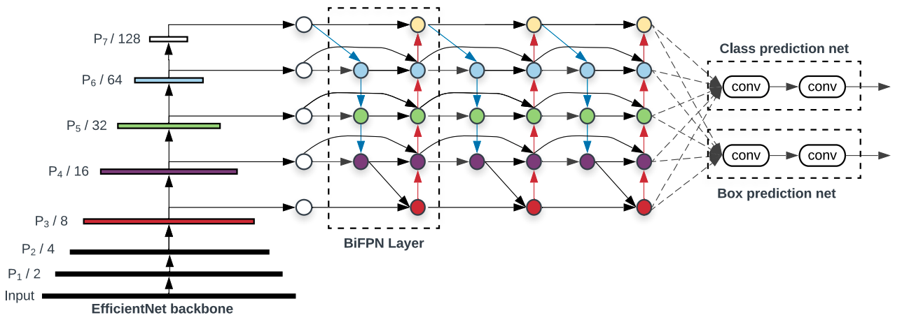
EfficientDet is a highly efficient and scalable object detection framework designed to maximize accuracy while minimizing computational costs. It achieves this by leveraging key innovations like the BiFPN (Bidirectional Feature Pyramid Network) for efficient multi-scale feature fusion and compound scaling to balance the resolution, depth, and width of the network components. EfficientDet’s ability to consistently outperform traditional object detection models like YOLOv3, RetinaNet, and Mask R-CNN across a wide range of resource constraints has made it a popular choice for object detection tasks.
However, while EfficientDet excels in general-purpose object detection, it is not well-suited for tasks like face recognition, which require identifying and differentiating between individual faces.
Multi-Scale Feature Fusion and Resource Bottleneck
EfficientDet’s BiFPN is optimized for detecting objects of varying sizes across different scales. It assigns learnable weights to feature maps at different resolutions, ensuring that objects as small as a few pixels or as large as an entire frame are accurately detected. This architecture is highly effective for detecting objects but introduces significant computational overhead, particularly when processing high-resolution inputs like face datasets. During training, this caused GPU memory usage to fluctuate heavily, peaking near capacity and occasionally crashing. The repeated top-down and bottom-up pathways in BiFPN, combined with the need to process multiple resolutions simultaneously, make it resource-intensive, especially for single-class detection tasks like faces.
Lack of Specialized Feature Encoding
Face recognition relies heavily on capturing fine-grained details and unique facial features that distinguish one individual from another. EfficientDet, being an object detector, focuses on localizing objects and classifying their presence rather than encoding discriminative details. Its feature maps are optimized for spatial localization and class prediction, not the subtle variations in facial landmarks needed for recognition. As a result, the extracted features lack the granularity required for high-accuracy face recognition tasks.
Overhead from Compound Scaling
EfficientDet uses a compound scaling method, which scales the resolution, depth, and width of the backbone, BiFPN, and prediction networks together. While this improves accuracy for general object detection, it significantly increases the computational cost when applied to high-resolution inputs, like face images. Training with larger batch sizes became infeasible in our setup due to memory constraints, forcing us to reduce the batch size and extend training time. The scaling, although efficient for diverse object detection, proved to be overkill for a single-object detection task like face detection, further limiting its practicality in resource-constrained environments.
Implementation
# 1. Modify the model to support the dataset
def get_model(num_classes):
    model = torchvision.models.detection.fasterrcnn_resnet50_fpn(weights="COCO_V1")
    in_features = model.roi_heads.box_predictor.cls_score.in_features
    model.roi_heads.box_predictor = FastRCNNPredictor(in_features, num_classes)
    return model

# 2. Faster training with AMP (Mixed Precision)
scaler = torch.cuda.amp.GradScaler()

def train_one_epoch(model, optimizer, data_loader, device, epoch, print_freq=50):
    model.train()
    loss_sum = 0.0
    for i, (images, targets) in enumerate(data_loader):
        images = [img.to(device) for img in images]
        targets = [{k: v.to(device) for k, v in t.items()} for t in targets]

        with torch.cuda.amp.autocast():  # Mixed precision
            loss_dict = model(images, targets)
            losses = sum(loss for loss in loss_dict.values())

        optimizer.zero_grad()
        scaler.scale(losses).backward()
        scaler.step(optimizer)
        scaler.update()

        loss_sum += losses.item()
        if (i + 1) % print_freq == 0:
            print(f"Epoch [{epoch}], Step [{i + 1}/{len(data_loader)}], Loss: {losses.item():.4f}")
    return loss_sum / len(data_loader)

# 4. Evaluation & visualization
def evaluate(model, data_loader, device):
    model.eval()
    with torch.no_grad():
        for images, targets in random.sample(list(data_loader), 1):  # Visualize one batch
            images = [img.to(device) for img in images]
            preds = model(images)

            for img, pred in zip(images, preds):
                visualize_image_and_bbox(img.cpu(), pred)

# Inference pipeline
def infer(model, image, device):
    model.eval()
    with torch.no_grad():
        image = image.to(device)
        pred = model([image])[0]  # Single image
        visualize_image_and_bbox(image.cpu(), pred)
    return pred

# Training setup
device = torch.device('cuda') if torch.cuda.is_available() else torch.device('cpu')
num_classes = 2  # Background + Face class
num_epochs = 10
batch_size = 4
learning_rate = 0.005

train_loader = DataLoader(train_dataset, batch_size=batch_size, shuffle=True,
                          collate_fn=lambda x: tuple(zip(*x)), num_workers=4, pin_memory=True)
model = get_model(num_classes).to(device)
optimizer = torch.optim.SGD(model.parameters(), lr=learning_rate, momentum=0.9, weight_decay=0.0005)
scheduler = StepLR(optimizer, step_size=3, gamma=0.1)

# Train
train_losses = []
start_time = time.time()
for epoch in range(1, num_epochs + 1):
    print(f"Epoch {epoch}/{num_epochs}")
    train_loss = train_one_epoch(model, optimizer, train_loader, device, epoch)
    train_losses.append(train_loss)
    scheduler.step()
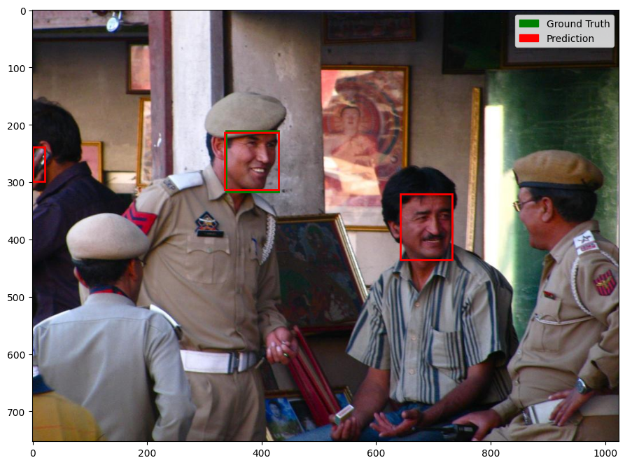
Observations
EfficientDet’s architecture is inherently optimized for detecting a variety of objects in complex scenes, making it ill-suited for specialized applications like face recognition, where task-specific architectures like FaceNet, ArcFace, or SphereFace excel. The resource-intensive nature of BiFPN and the lack of a focus on encoding identity-specific features render EfficientDet impractical for face recognition tasks. After training this model and evaluating it, we were able to achieve a mean IoU of \(0.47\), a lower measure compared to the other models used in this project.
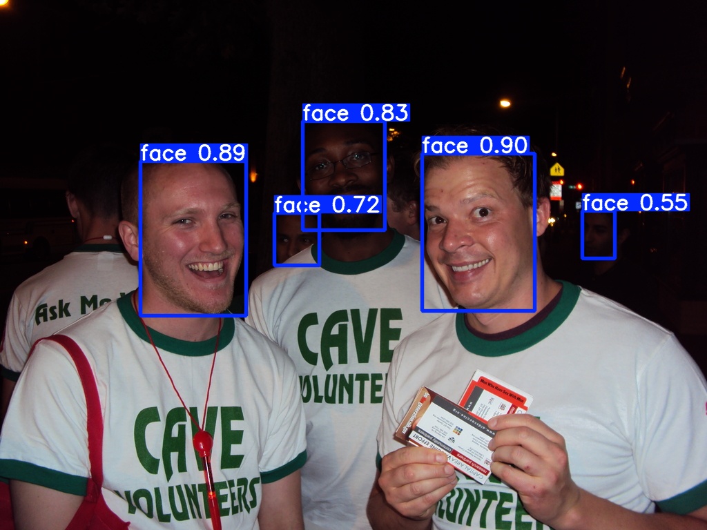
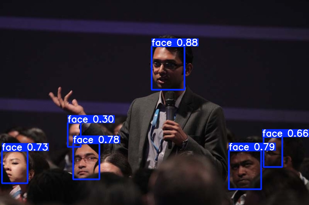
Example Model Outputs
| Faster R-CNN, SSD, EfficientDet | YOLOv5 |
|---|---|
 |
 |
 |
 |
 |
 |
Final Words & Conclusion
In this project, we examined the performance of four modern object detection models for facial recognition tasks, each with its unique strengths and limitations. Faster R-CNN demonstrated exceptional accuracy but struggled with inference speed, making it less suitable for real-time applications. SSD offered a balanced trade-off between speed and accuracy, while YOLOv5 stood out for its efficiency and real-time capabilities. Lastly, EfficientDet showcased scalability and multi-scale detection but proved less practical for face-specific tasks due to its computational overhead.
Our findings emphasize that the choice of a model depends heavily on the application requirements, including the need for speed, accuracy, and resource constraints. By understanding these trade-offs, practitioners can make informed decisions when deploying facial recognition systems.
Reference
[1] Ren et al. “Faster R-CNN: Towards Real-Time Object Detection with Region Proposal Networks”. https://arxiv.org/abs/1506.01497v3. 2016.
[2] Li et al. “SSD7-FFAM: A Real-Time Object Detection Network Friendlyto Embedded Devices from Scratch”. https://www.researchgate.net/publication/348769625_SSD7-FFAM_A_Real-Time_Object_Detection_Network_Friendly_to_Embedded_Devices_from_Scratch. 2021.
[3] Tsang, Sik-Ho. “Brief Review: YOLOv5 for Object Detection”. https://sh-tsang.medium.com/brief-review-yolov5-for-object-detection-84cc6c6a0e3a. 2023.
[4] Tan et al. “EfficientDet: Scalable and Efficient Object Detection”. https://arxiv.org/abs/1911.09070v7. 2019.
[5] Skelton. “Faster R-CNN Explained for Object Detection Tasks”. https://www.digitalocean.com/community/tutorials/faster-r-cnn-explained-object-detection. 2024.
[6] Liu et al. “SSD: Single Shot MultiBox Detector”. https://arxiv.org/abs/1512.02325. 2015.
[7] Forson. “Understanding SSD MultiBox — Real-Time Object Detection In Deep Learning”. https://towardsdatascience.com/understanding-ssd-multibox-real-time-object-detection-in-deep-learning-495ef744fab. 2017.
[8] Khanam et al. “What is YOLOv5: A deep look into the internal features of the popular object detector”. https://arxiv.org/abs/2407.20892, 2024.