CNN Loss Function Advances for Deep Facial Recognition
In this report, we focus on analyzing loss functions used in Convolutional Neural Networks (CNNs) for Deep Face Recognition, specifically comparing A-Softmax, CosFace, and ArcFace, and examining their performances.
Introduction
We will be focusing on loss functions used in CNNs for Deep Face Recognition, and analyzing their performances.
Facial recognition tasks rely on computer vision to identify or group people in images or videos. The source for the input image can be a phone camera, security cameras, or drones, among other sources. The initial pioneers of facial recognition, Woody Bledsoe, Helen Chan Wolf, and Charles Bisson, manually marked key human features and fed them into machines in the 1960s. Now, with the field bolstered by the recent boom in computer vision, models for facial recognition have steadily improved. In one way or another, most individuals with a smartphone are exposed to facial recognition every day through their photo management applications or FaceID.
Despite the advances made in this field, some challenges remain. Maintaining accuracy of the model even with variations in lighting, pose, or expressions is an existing obstacle to be tackled. Some images that have occlusion, low resolution, or partial face block can also cause problems. Questions of the ethics of FR, potentially jeopardized security of the sensitive databases amassed for this specific task, and racial/ethnic bias are all important issues that must be taken into account when developing a model for facial recognition. For this report, the main focus will be on the improvement of facial recognition models, specifically the loss functions implemented in many of the deeper CNN models.
A-Softmax
A-Softmax is a loss function based on Softmax. The key difference is that it projects the Euclidean space into an angular space to incorporate an angular margin. The angular margin is preferred because the cosine of the angle aligns better with the concept of softmax.
Loss function:
\(L = \frac{1}{N} \sum_{n=1}^{N} -\log {\frac{e^{\left\| \textbf{x}^{(n)} \right\|\Phi(\Theta^{(n)}_{y_{n}})}}{e^{\left\| \textbf{x}^{(n)} \right\|\Phi(\Theta^{(n)}_{y_{n}})} + \sum_{ j \neq{y_{}}}^{n} e^{\left\| \textbf{x}^{(n)} \right\|cos(\Theta_{j}^{(n)})}}}\)
\(\Phi(\Theta^{(n)}_{y_{n}}) = (-1)^{k}cos(m\Theta_{y_{n}}^{(n)})-2k\)
Where N is the number of training samples.
Testing Protocols for Facial Recognition
To test a model of facial recognition, there are two settings: either closed-set or open-set. A closed-set protocol would have all testing identities predefined in the training set, making the facial recognition class one of a classification problem. On the other hand, open-set protocols have testing identities that are separate from the training set. This makes open-set FR more difficult to achieve but is in practice closer to real life applications. In open-set protocols, classifying the faces to known identities in the training set is not possible, so the faces must be mapped to a discriminative feature space. The end goal of open-set facial recognition is to learn discriminative large-margin features.
Enhancement of Discriminative Power
For the model to work as desired, it is necessary for the intra-class variation of faces to be smaller than the inter-class distance between faces to get good accuracy using the nearest neighbor algorithm. Before the work of Liu et. al in their paper SphereFace: Deep Hypersphere Embedding for Face Recognition, CNN-based models could not effectively satisfy these requirements. The commonly chosen loss function, the softmax function, was not able to learn separable features that were discriminative enough. Previous models imposed Euclidean margins to learned features, while the authors of this paper introduced incorporating angular margins instead.
A-Softmax Loss
The decision boundary in softmax loss is
\((\textbf{W}_{1} - \textbf{W}_{2})\textbf{x} + b_{1} - b_{2} = 0\)
where Wi and bi are the weights and bias.
Define x as a feature vector, and constrain:
\(\left\| \textbf{W}_{1} \right\| = \left\| \textbf{W}_{2} \right\| = 1\)
and b1 - b2 = 0
Decision boundary becomes:
\(\left\| \textbf{x} \right\|(cos(\Theta_{1})- cos(\Theta_{2})) = 0\)
where theta is the angle between Wi and x. This new decision boundary only depends on theta, and is able to optimize angles directly. This helps the CNN to learn the angularly distributed features. However, this is not enough to increase the discriminative power of the features. The integer m is introduced to quantitatively control the size of the angular margin.
In binary-class case:
Class 1 Decision Boundary:
\(\left\| \textbf{x} \right\|(cos(m\Theta_{1})- cos(\Theta_{2})) = 0\)
Class 2 Decision Boundary:
\(\left\| \textbf{x} \right\|(cos(\Theta_{1})- cos(m\Theta_{2})) = 0\)
When A-softmax loss is optimized, the inter-class margin is enlarged at the same time as the intra-class angular distribution is compressed, leading to the decision regions to be more separated. Existing CNN architectures have been shown to benefit from A-Softmax loss and its ability to learn discriminative face features. Liu et. al were the first to show the effectiveness of this angular margin introduction in facial recognition. Below is a figure from the published article that showcases the difference in accuracy between A-Softmax and Softmax on the Labeled Face in the Wild (LFW) and YouTube Faces (YTF) datasets.
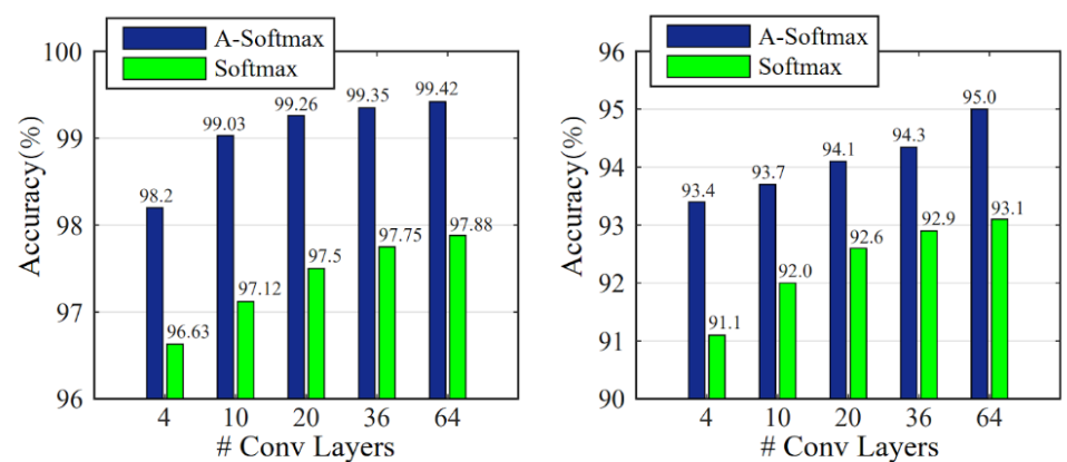
Fig 1. Comparison of accuracies of A-Softmax and Softmax with varying numbers of convolution layers [7].
A-Softmax loss lends a useful geometric interpretation for discriminative learned features, and after the introduction of it with this paper, has been implemented in other areas by computer vision researchers in the field of facial recognition, primarily CosFace and ArcFace.
CosFace
CosFace is a model proposed in 2018 that uses a novel loss function called large margin cosine loss (LMCL) instead of the widely used softmax loss. This loss function is designed to improve upon the discriminating power of previous loss functions, such as the original softmax loss and A-Softmax loss. It focuses on having a large inter-class angular margin in order to strengthen the discriminating power. The overall framework of the CosFace model is visualized in Figure 2.
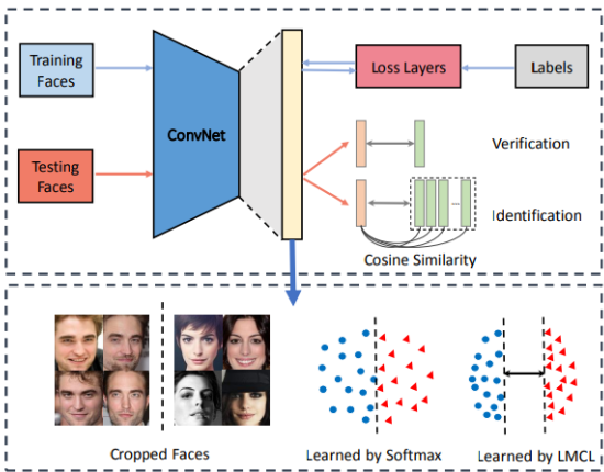
Fig 2. An overview of the proposed CosFace framework [2].
Loss function:
Like A-Softmax, LMCL works in the angular space instead of the Euclidean space. It modifies the traditional softmax loss by normalizing feature and weight vectors using L2 normalization to eliminate radial variability. Additionally, a cosine margin is added to strengthen the decision boundary within the angular domain. The loss is defined by:
where N is the number of training samples, xi is the i-th feature vector corresponding to the ground-truth class of yi, the Wj is the weight vector of the j-th class, and theta_j is the angle between Wj and xi. The cosine margin m is defined such that the LMCL decision boundary is given by:
\(\cos{(\theta_1)}-m = \cos{(\theta_2)}\)
The decision margin is defined in the cosine space, which solves the issue of having different margins for different classes like A-Softmax. The decision boundaries of Softmax, A-Softmax, and LMCL are visualized in Figure 3.
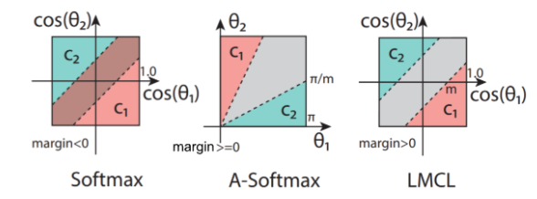
Fig 3. The comparison of decision margins for different loss functions in the binary-classes scenarios. Dashed lines represent the decision boundary, and gray areas are decision margins. [2].
Normalization
Both the weight vectors and feature vectors are normalized in LMCL. Feature normalization removes radical variance, which increases the model’s discriminative power. Without normalization, the original softmax loss jointly learns the Euclidean norm (L2-norm) of feature vectors and their angular relationships, which weakens the focus on angular discrimination. By enforcing a consistent L2-norm across all feature vectors, the learning process depends solely on cosine values, effectively clustering features of the same class and separating those of different classes on a hypersphere.
CosFace was trained on the small dataset CASIA-WebFace, with a CNN architecture consisting of 64 convolutional layers, both with and without normalization. It was then tested on several public face datasets, including LFW, YTF, and MegaFace. The results are shown in Table 1. The model with normalization performed with better accuracy than the model that skipped the normalization step in all three datasets.
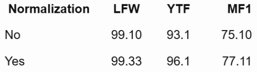
Table 1. Comparison of LMCL with and without feature normalization. [2].
Cosine Margin m
The value of m plays an important role in improving learning of highly discriminable features. A higher value of m enforces a stricter classification, making the learned features more robust against noise. On the other hand, too large an m prevents the model from converging since the cosine constraint
becomes too hard to satisfy. The bounds of m turn out to be
\(0 \leq m \leq 1-\cos{(\frac{2 \pi}{C})}, (K=2)\)
\(0 \leq m \leq \frac{C}{C-1}, (C \leq K+1)\)
\(0 \leq m \ll 1\frac{C}{C-1}, (C > K+1)\)
where C is the number of training classes and K is the dimension of the learned features. In an experiment with 8 distinct identities (8 faces), the upper limit of m would be:
In Figure 4, three valid values of m were tested and compared against each other as well as against the performance of Softmax. The first row maps the features on the Euclidean space, while the second row projects the features onto the angular space.
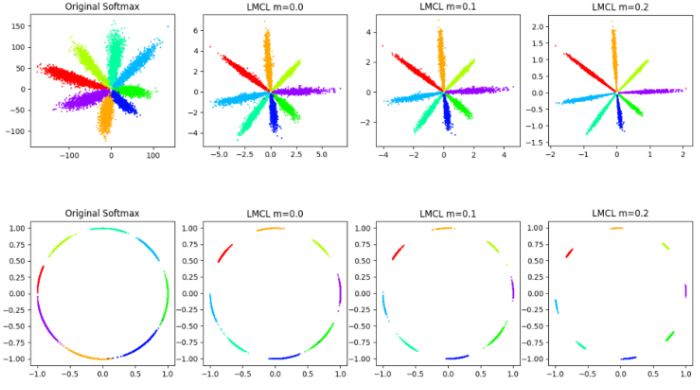
Fig 4. A toy experiment of different loss functions on 8 identities, comparing Softmax and LMCL [2].
The values of m, ranging from 0 to 0.45, were tested on the datasets LFW and YTF. The upper limit was set to 0.45 because with the dataset, 0.45 was the point of no convergence. As the value of m increased, the accuracy of the model also increased up until m=0.35, when the performance began to decline.
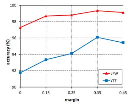
Fig 5. Comparing the accuracy of CosFace with different values of m [2].
ArcFace
CosFace was able to improve on the loss function to obtain better performance while also offering easier implementation. Efforts to further improve loss functions for facial recognition models culminated in the development of ArcFace, proposed by Deng et. al in their paper ArcFace: Additive Angular Margin Loss for Deep Face Recognition. ArcFace uses another loss function, Additive Angular Margin Loss, to stabilize the training process and improve the discriminative power of recognition model. This loss function adds an additive angular margin penalty m. ArcFace optimizes the geodesic distance margin, and achieves excellent performance on multiple face recognition benchmarks, on both image and video datasets. It is both easy and efficient to implement, only needing a few lines of code and does not add high levels of computational complexity during training.
Loss function:
\(L_{aam} = - \frac{1}{N} \sum_{i=1}^{N} \log {\frac{e^{s( \cos{(\theta_{yi}+m)})}}{e^{s( \cos{(\theta_{yi}+m)})} + \sum_{j=1, j \neq{y_i}}^{n} e^{s \cos{\theta_j}}}}\)
A toy experiment similar to the one run for CosFace was run for ArcFace. The comparison of the results against Softmax is shown in Figure 5. The classes are clearly separated with ArcFace, a significant improvement from Softmax where the classes tend to blend together at the decision boundaries.
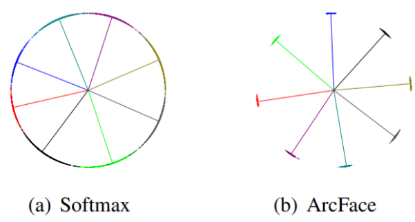
Fig 6. A toy experiment of different loss functions on 8 identities. Comparison between Softmax and ArcFace. [3].
ArcFace was evaluated on the widely used benchmark datasets Live Faces in the Wild (LFW) and YouTube Faces (YTF) as well. ArcFace that was trained on MS1MV2 (a database featuring mainly celebrities) beat the baseline for CosFace with a significant margin. It proved more accurate than many of the other available methods, as depicted in Figure 7.
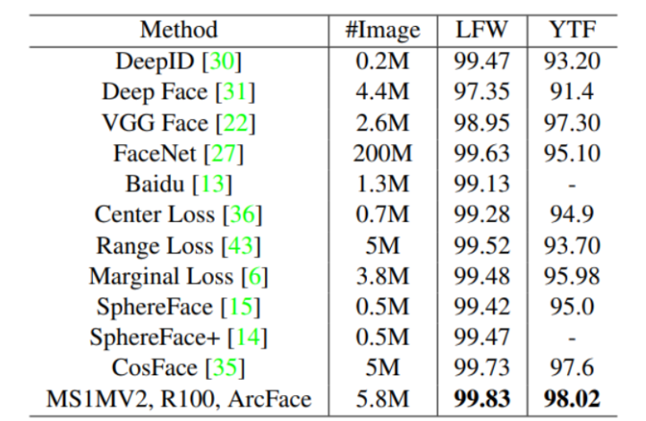
Fig 7. Performance comparison of different methods on LFW and YTF, featuring ArcFace outperforming all of them. [3].
Results & Experiments
Running Existing Codebase
I ran an existing Google Collab notebook that illustrated a basic arc face loss example. Here is the implementation of arcface:
class AdditiveAngularMarginPenalty(nn.Module):
    """
        Insightface implementation : https://github.com/deepinsight/insightface/blob/master/recognition/arcface_torch/losses.py
        ArcFace (https://arxiv.org/pdf/1801.07698v1.pdf):
    """
    def __init__(self, s=64.0, margin=0.5):
        super(AdditiveAngularMarginPenalty, self).__init__()
        self.s = s
        self.margin = margin

        self.cos_m = math.cos(margin)
        self.sin_m = math.sin(margin)
        self.theta = math.cos(math.pi - margin)
        self.sinmm = math.sin(math.pi - margin) * margin
        self.easy_margin = False

    def forward(self, logits: torch.Tensor, labels: torch.Tensor):
        index = torch.where(labels != -1)[0]
        target_logit = logits[index, labels[index].view(-1)]

        with torch.no_grad():
            target_logit.arccos_()
            logits.arccos_()
            final_target_logit = target_logit + self.margin
            logits[index, labels[index].view(-1)] = final_target_logit
            logits.cos_()
        logits = logits * self.s
        return logits
Here is the implementation of the basic model:
class ToyMNISTModel(nn.Module):
  def __init__(self):
    super(ToyMNISTModel, self).__init__()

    self.conv1 = nn.Conv2d(1, 32, 5)
    self.conv2 = nn.Conv2d(32, 32, 5)
    self.conv3 = nn.Conv2d(32, 64, 5)
    self.dropout = nn.Dropout(0.25)
    self.fc1 = nn.Linear(3*3*64, 256)
    self.fc2 = nn.Linear(256, 10)
    self.angular_margin_penalty = AdditiveAngularMarginPenalty(10, 10)
    self.relu = nn.ReLU(inplace=True)
    self.maxpooling = nn.MaxPool2d(2, 2)

  def forward(self, x, label=None):
    # CNN part
    x = self.relu(self.conv1(x))
    x = self.dropout(x)
    x = self.relu(self.maxpooling(self.conv2(x)))
    x = self.dropout(x)
    x = self.relu(self.maxpooling(self.conv3(x)))
    x = self.dropout(x)

    # fully connected part
    x = x.view(x.size(0), -1)    # (batch_size, 3*3*64)
    x = self.relu(self.fc1(x))
    x = self.fc2(x)

    if label is not None:
      # angular margin penalty part
      logits = self.angular_margin_penalty(x, label)
    else:
      logits = x

    return logits
Running this notebook, I got these image feature visualizations after training with Arcface:
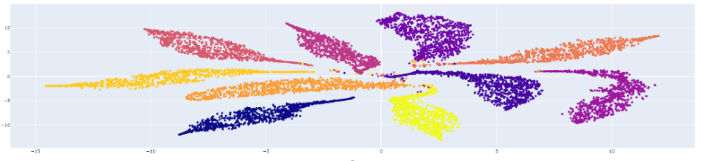
Fig 8. Image Feature Visualization with ArcFace. [1]
Compared to running the same model with normal softmax, I got this:
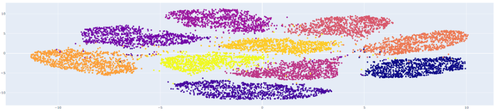
Fig 9. Image Feature Visualization without ArcFace (Softmax) [1]
The first visualization (ArcFace) is preferable because it demonstrates better separation between the feature clusters corresponding to different classes.
Link to the Existing Codebase I ran
Implementing Our Own ideas
After running the existing notebook, I decided to run the deepface module myself for arc face. I compared the results for different models, such as Facenet and VGG-Face. Having tested it on a few images that I uploaded, I got very similar results compared to other models. However, looking at the thresholds and differences, I noticed that Arcface tends to be more strict and penalizes differences more compared to the other models. This made it less likely to have false positives.
Collab Notebook Link for Implementing our Own Ideas
Reference
[1] Shizuya, Y. (2024, June 27). ArcFace — Architecture and Practical example: How to calculate the face similarity between images. Medium. https://medium.com/@ichigo.v.gen12/arcface-architecture-and-practical-example-how-to-calculate-the-face-similarity-between-images-183896a35957
[2] Wang, H. et al. “CosFace: Large Margin Cosine Loss for Deep Face Recognition.” 2018.
[3] Deng, Jiankang et al. “ArcFace: Additive Angular Margin Loss for Deep Face Recognition” Proceedings of the IEEE conference on computer vision and pattern recognition. 2019.
[4] Nayeem, M. (2020, September 27). ArcFace based Face recognition. Analytics Vidhya. https://medium.com/analytics-vidhya/exploring-other-face-recognition-approaches-part-2-arcface-88cda1fdfeb8
[5] Papers with code - ArcFace explained. (n.d.). Papers With Code. Retrieved December 13, 2024, from https://paperswithcode.com/method/arcface
[6] Zafeiriou, J. D., Jia Guo, Niannan Xue, Stefanos. (n.d.). ArcFace: Additive angular margin loss for deep face recognition.
[7] Liu, W. et al. “SphereFace: Deep Hypersphere Embedding for Face Recognition”. 2017