Face Detection: From Neural Networks to Dense Detectors
The field of face detection has evolved significantly from early neural network approaches to modern deep learning architectures. This article traces this evolution, focusing particularly on Deep Dense Face Detector (DDFD). We examine how DDFD built upon earlier foundations like Rowley’s neural networks and the Viola-Jones framework while introducing innovations that enabled face detection across multiple views without requiring pose annotations. The paper analyzes DDFD’s architectural choices, training methodology, and performance characteristics compared to contemporary approaches like R-CNN. We highlight DDFD’s practical applications through case studies, including its integration into face detection and tagging systems achieving 85% accuracy.
- Introduction
- Early Neural Network Approaches
- Viola-Jones Framework
- Deep Dense Face Detector
- Comparing R-CNN to DDFD
- DDFD in Practice: Extension to Face Detection and Tagging Systems
- Running Code
- Conclusion
- References
Introduction
Face detection has undergone a remarkable transformation over the past few decades, evolving from simple neural networks to sophisticated deep learning architectures. The journey began with Rowley et al.’s pioneering work in 1998 [1], which introduced fundamental concepts like neural network-based classification, bootstrap training, and network arbitration. While revolutionary, this early approach struggled with variations in pose and lighting. The field’s next major breakthrough came with the Viola-Jones detector in 2001 [2], achieving real-time detection through integral images, AdaBoost feature selection, and cascaded architecture. Despite its practical success, Viola-Jones remained primarily effective only for frontal faces. Deep Dense Face Detector (DDFD) then represented a paradigm shift by leveraging convolutional neural networks to detect faces across multiple views without requiring pose annotations, achieving superior accuracy while maintaining reasonable computational efficiency compared to methods like Deformable Part Models (DPM).
When compared to Region-based CNN (R-CNN), DDFD occupies an important middle ground in the evolution of face detection. While R-CNN methods achieve high accuracy through region proposals, they require significant computation, whereas DDFD’s sliding window approach offers better practical efficiency [3]. Looking ahead, face detection continues to evolve toward real-time mobile performance, integration with other facial analysis tasks, and addressing bias concerns in practical applications. The progression from Rowley’s neural networks through DDFD to modern approaches illustrates how advances in computing power, architectural innovations, and machine learning techniques continuously push the boundaries of computer vision capabilities.
Early Neural Network Approaches
The work of Rowley et al. in 1998 showed that neural networks could effectively detect faces by examining small windows of an image [1]. They used a retinally-connected neural network examining 20x20 pixel windows. These were connected to multiple networks to improve performance. A bootstrap training algorithm was used to select negative examples with heuristics to merge overlapping detections. While this early work is definitely dated in its approach, it established key principles such as using neural networks for binary classification which was lesser known at the time. It also develops the process of bootstrap training on hard negatives, arbitration between multiple detectors, and detection at multiple scales. A key innovation in Rowley’s work was the training methodology, particularly for handling negative examples. Rather than trying to manually select a representative set of nonface training examples, which would be an impossible task given the vast space of possible nonface images, they developed a bootstrap training approach. The network was initially trained on a small set of face and random nonface examples and then applied to images of scenery containing no faces. False detections were collected and added back into the training set. This iterative process allowed the network to automatically focus on the most challenging negative examples that were similar enough to faces to cause confusion. The network contained three types of hidden units: 4 units examining 10x10 pixel subregions, 16 units looking at 5x5 pixel regions, and 6 units analyzing overlapping 20x5 pixel horizontal stripes. These different receptive field sizes allowed the network to detect both local features like individual facial features as well as more holistic horizontal patterns characteristic of faces.
Early Network Architecture
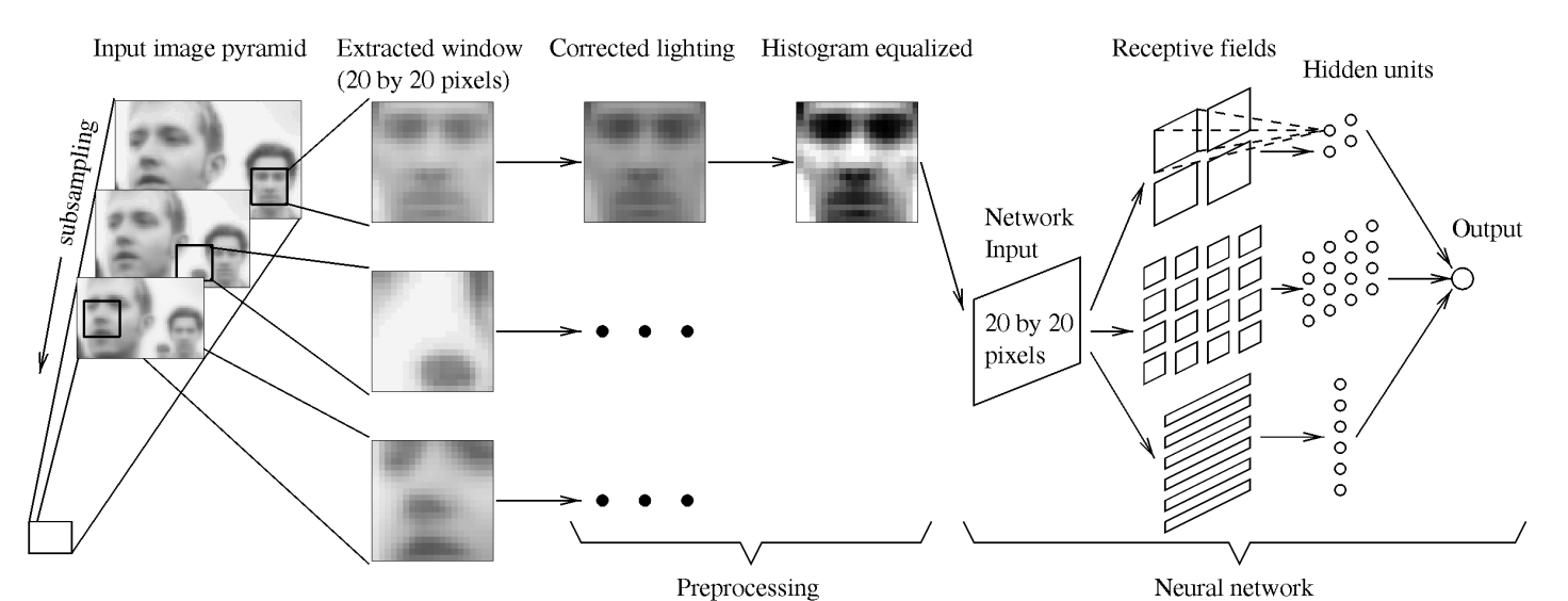
Fig 1. Network Architecture from Rowley [1].
When compared to contemporary systems of the time, Rowley’s neural network approach achieved state-of-the-art detection rates while running at reasonable speeds on late 1990s hardware, processing a 320x240 pixel image in around 2-4 seconds.
Viola-Jones Framework
The Viola-Jones detector represented a major advance with key innovations such as integral image representation, the inclusion of AdaBoost for feature selection, using a cascaded architecture and Haar-like features to improve efficiency and computation speeds. The Viola-Jones detector, introduced in 2001, revolutionized face detection by being the first real-time face detection system capable of processing images at 15 frames per second [2]. They introduced integral image representation, which allowed for extremely fast computation of Haar-like features. An integral image could be computed in a single pass over an image, after which any rectangular sum could be computed with only four array references. This enabled calculating a large number of rectangular features efficiently.
Another fundamental contribution was the usage of AdaBoost for both feature selection and classifier construction. The classifier construction is as follows:
\[C(x) = \begin{cases} 1 & \text{if } \sum_j h_j(x) > T \\ 0 & \text{otherwise} \end{cases}\]AdaBoost combined many “weak” classifiers (each based on a single Haar-like feature) into a strong classifier by iteratively selecting features and adjusting their weights based on their performance on the training set, automatically selecting the most discriminative features.
Viola-Jones also introduced a cascaded architecture, improving computational efficiency while maintaining high detection accuracy. The cascade consisted of increasingly complex stages of classifiers, where each stage quickly rejected obvious non-face regions and passed potential face regions to later more complex stages for detailed analysis. Early stages used very few features (as few as 2) and could rapidly reject the majority of non-face windows, while later stages used more features (up to 200) to achieve high accuracy on harder examples. This cascaded architecture meant that most computation was focused on promising face-like regions, while obvious non-faces were rejected with minimal computation.
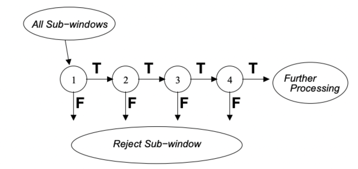
Fig 2. Viola Jones Logic Flow [2].
This is a schematic representation of the cascaded architecture which rejected more obvious sub-windows in earlier stages, leading to less computation and processing; later stages eliminate more negatives at a higher processing rate.
The efficiency of the integral image representation combined with the cascade structure enabled the first real-time face detector, fundamentally changing what was possible in face detection applications.
Deep Dense Face Detector
Overview
Deep Dense Face Detector (DDFD) represented a significant advance in face detection by introducing a single CNN architecture capable of handling multi-view face detection without requiring pose annotations or multiple models. The network uses an architecture similar to AlexNet, with five convolutional layers followed by three fully connected layers. The key innovation is in how DDFD processes images - rather than requiring region proposals like R-CNN or specialized pose-specific models, it applies the CNN directly through a sliding window approach across multiple scales. This design choice makes DDFD both simpler and more efficient than contemporary approaches, while still achieving good detection rates.
Training and Experimental Process
For face detection training, training examples were extracted from the AFLW dataset, which consists of 21K images with 24K face annotations. To increase the number of positive examples, sub-images were randomly sampled and classified as positive if the Intersection over Union (IoU) score (with the ground truth) was 50% over higher. The training examples were also flipped. After data augmentation, there were 200K positive examples and 20 million negative examples. The neural network was fine-tuned on Alex-Net, using a batch size of 128 images (with 32 positive examples and 96 negative examples each) and 50K iterations. To tune the hyperparameters, the PASCAL Face dataset (851 images with 1341 annotated faces) was used.
Different scaling factors were tested to enable the model to scan images in finer detail, but this also increased the computation time.
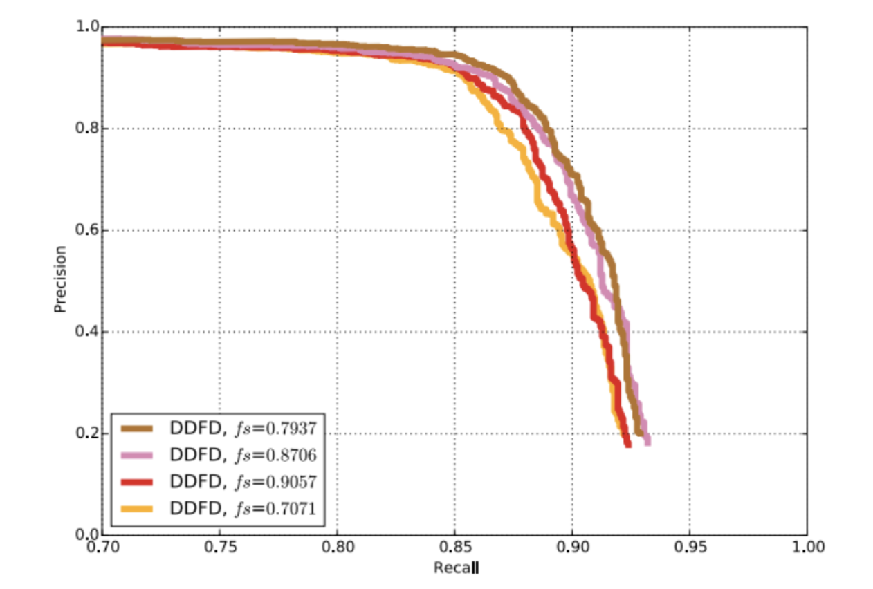
Fig 3. Effect of scaling factor on precision and recall of the detector. [3].
Two strategies using Non-Maximal Suppression were used: NMS-max and NMS-avg, with NMS-avg outperforming NMS-max.
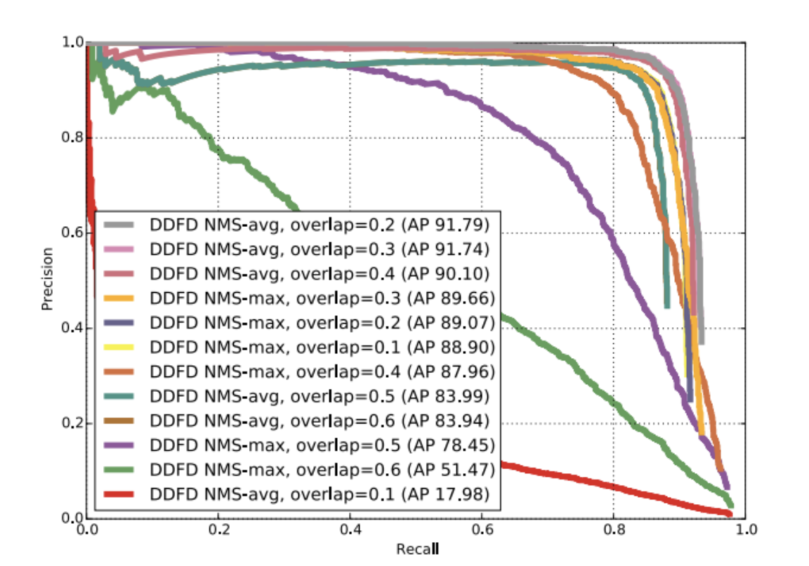
Fig 4. Effect of different NMS strategies and their overlap thresholds. [3].
Lastly, bounding-box regressors were trained to improve detector localization. The regressors predicted the mismatch between the ground truth and bounding boxes generated by the model. However, the regressors combined with the NMS strategies worsened the overall performance of the model. This was because of side-view face annotation mismatches between the training and testing tests.
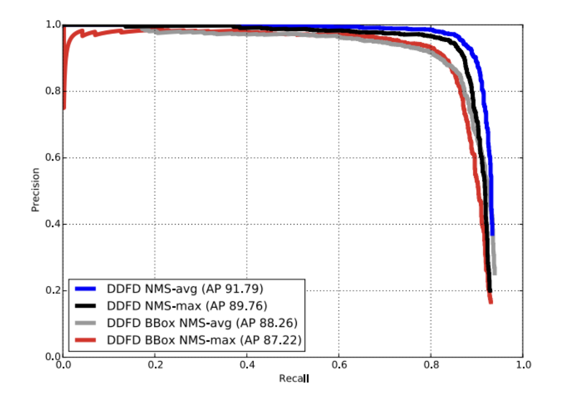
Fig 5. Performance of the proposed face detector with and without bounding-box regression. [3].
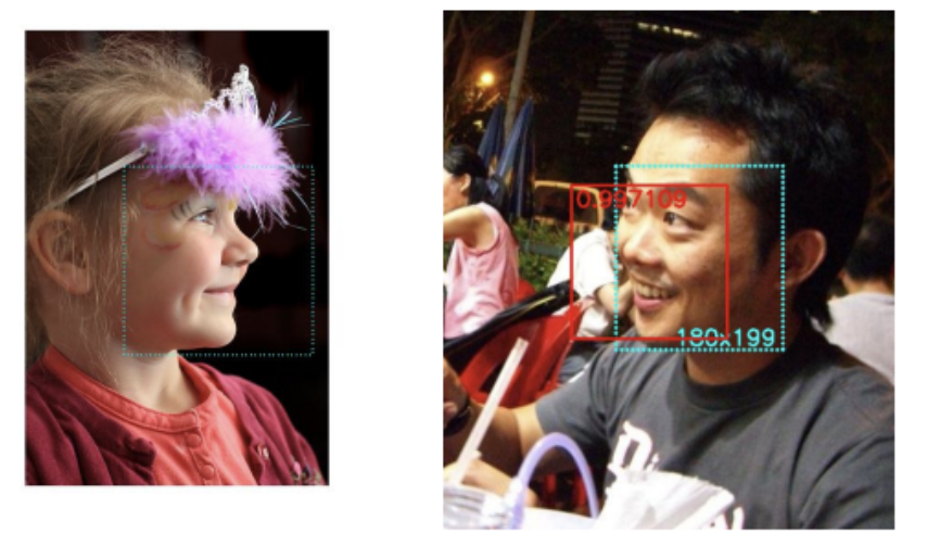
Fig 6.Annotation of a side face in left) training set and right) test set. The red bounding-box is the predicted bounding-box by our proposed detector. This detection is counted as a false positive as its IOU with ground truth is less than 50%. [3].
Testing
To test the model, a combination of datasets of PASCAL, AFW (205 images with 473 annotated faces), and FDDB (2846 images with 5171 annotated faces) were used. These datasets had images with occluded, low-resolution and/or out-of-focus, with cluttered backgrounds and large variations in angles and physical appearance. The bounding-box regressors were used at test time to adjust the bounding-box to predict the location of faces more accurately.
Comparing R-CNN to DDFD
R-CNN is one of the most commonly used object detection methods. The main difference between R-CNN and DDFD is the intended application of the frameworks. R-CNN is an adaptable framework and intended for general purpose object detection tasks, as referenced in Girshick, Ross, et al [4]. In R-CNN, the modularity between region proposal generation, feature extraction, and classification allows for greater flexibility to modify the general components without having to change every part of the model. The pool5 features in CNN are learned from large data, such as ImageNet, which provides general features that allow domain specific fine-tuning at the higher layers. This allows for feature flexibility that makes R-CNN modular. On the other hand, DDFD is specialized for face detection. A sliding window approach is used to obtain the final face detector. The confidence of each face detection is then shown in a heatmap. This dense feature abstraction works well for faces because facial structure is consistent amongst most variations, but will not work well for general object detection. In addition to this, DDFD simplifies its architecture, getting rid of components not necessary for facial detection.
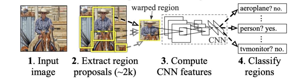
Fig 7.Comparison of our face detector, DDFD, with different R-CNN face detectors. [3].
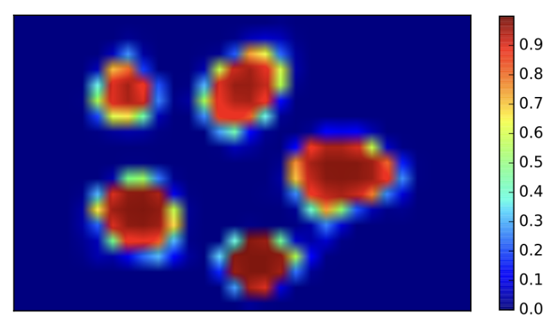
Fig 8.Comparison of our face detector, DDFD, with different R-CNN face detectors. [3].
When comparing R-CNN to DDFD, there are fundamentally different approaches to detecting. R-CNN relies on around 2,000 region proposals per image that are generated from high capacity convolutional neural networks [4]. This is followed by feature extraction and SVM classification. DDFD uses a sliding window approach to apply the CNN. When looking at the generated heat map above, scores are all close to zero in regions that do not have a detected face [3]. This means DDFD has strong discriminative power and output can be used directly (no SVM or post-processing steps). In addition to this, R-CNN uses bounding box regression to reduce mislocalizations. On the other hand, when using a simple bounding box regression module in DDFD, it degraded performance making DDFD much simpler than R-CNN.
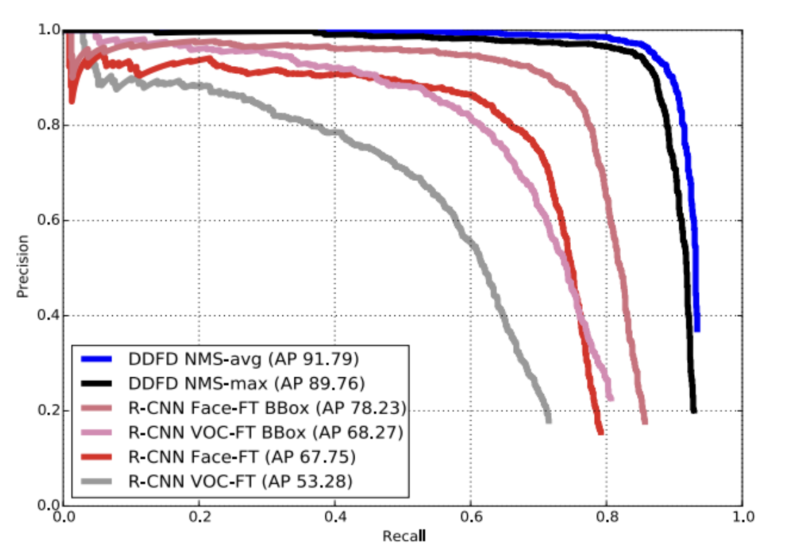
Fig 9.Comparison of face detector, DDFD, with different R-CNN face detectors. [4].
This architectural difference has significant implications for both accuracy and efficiency. Overall, R-CNN achieves a mAP of 53.7% on PASCAL VOC 2010 dataset [4]. In order to compare the performance to DDFD, the R-CNN model can be trained specifically for face recognition. The above graph shows DDFD with various NMS strategies and R-CNN with AlexNet fine tuned for different data (Face-FT and PASCAL VOC 2012). When training R-CNN for facial data using a bounding box, it performs the best, however it still does not have precision as high as DDFD. In addition to the precision, DDFD has an improved efficiency compared to R-CNN. As discussed previously, DDFD has streamlined architecture, specifically for facial recognition, allowing certain steps that R-CNN does to be skipped in DDFD.
DDFD in Practice: Extension to Face Detection and Tagging Systems
In discussing DDFD’s impact and applications, one notable example comes from Mehta et al.’s 2018 work that extended DDFD into a complete face detection and tagging system [5]. Their work demonstrates how DDFD’s core architecture can be effectively integrated into larger computer vision pipelines while maintaining its key advantages in handling multi-view face detection. Out of the faces detected by DDFD, their network was able to correctly tag 85% of those images.
Like DDFD, the face detecting process started by fine-tuning AlexNet with batch training of size 128 images for 50K iterations. They used a custom data set with 1500 images, rescaling each image to be 227 x 277. They passed images through DDFD to generate a heat-map indicating the location of the detected faces:
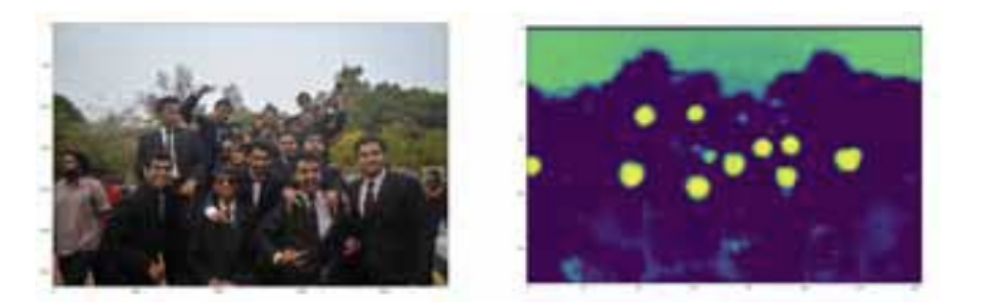
Fig 10. An example of generating a heat-maps using CNN [4].
To tag the face, Mehta et al. trained models for each face, using Local Binary Patterns Histograms (LBPH) method to analyze and classify the faces. The tagging system uses an algorithm to pass the detected faces into the trained models. Once a match is found, the face is tagged with the label.

Fig 11. Tagged image for entered input [4].
The system was able to maintain strong performance for detecting and tagging images under challenging conditions: partial occlusion, varied orientations and low resolution - all key strengths of the original DDFD approach. The results particularly highlight DDFD’s robustness in real-world applications and validates its adaptability, demonstrating how DDFD can be customized for specific applications while maintaining its core functionality.
The performance was measured with precision, recall and F-measure (harmonic mean of precision and recall).
\[\text{Precision}(P) = \frac{\text{Number of relevant items retrieved}}{\text{Number of retrieved items}}\] \[\text{Recall}(R) = \frac{\text{Number of relevant items retrieved}}{\text{Number of relevant items}}\] \[\text{F-measure} = \frac{2PR}{P + R}\]Results for Face Tagging
| Dataset Name | True Pos. | True Neg. | False Pos. | False Neg. | Prec. | Recall | F-mean |
|---|---|---|---|---|---|---|---|
| MIT Manipal Farewell 2017 | 480 | 150 | 100 | 70 | 82.75% | 85.7% | 84.18% |
| Custom Different Oriented Faces | 631 | 150 | 129 | 109 | 83.02% | 85.27% | 84.12% |
| Randomly Selected Celebrities | 949 | 210 | 142 | 189 | 86.98% | 83.39% | 84.14% |
Running Code
To explore DDFD in more detail we took a look at code samples online replicating the architecture. One example we found was created by Jakub Kolodziejczyk [5]. Kolodziejczyk’s work is based on “Multi-view Face Detection Using Deep Convolutional Neural Networks” by Farfade et al., [3] although some implementation details did differ. The implementation used the the Large-scale CelebFaces Attributes (CelebA) Dataset.
We attempted to run the code however due to some issues with obtaining the right packages and downloading the data we decided to instead use the implementation as reference and build a simpler model that detects faces.
We present two architectures DDFD (simplified) and ImprovedDDFD (an improvement based on our original DDFD implementation).
Deep Dense Face Detector (DDFD)
The DDFD model we built employs a CNN architecture that is optimized specifically for face detection. We built this model using AlexNet as the backbone, and leveraging PyTorch. The simplified DDFD model uses conv1-5 for feature extraction (reused from AlexNet). The binary classification between face and not face is achieved with a modified classifier. This modified classifier uses dropout, ReLU activations, fully connected layers and a sigmoid layer that outputs probabilities. The model is trained on the CelebA dataset, using binary cross entropy loss and SGD optimizer with momentum. When training the simplified DDFD mode, we achieved a validation accuracy of around 66%.
ImprovedDDFD
Building upon the foundational DDFD, the ImprovedDDFD incorporates advanced training methodologies, including better data augmentation and balanced sampling techniques. The improved DDFD model is built with ResNet18 as the backbone for feature extraction. A custom classifier is used for binary classification, implementing adaptive average pooling, ReLU, dropout, and sigmoid. To train the model, curriculum learning is used. In addition to this, the dataset is augmented with hard negative mining, generating negative examples through techniques like background cropping, partial face cropping and geometric transformations. Binary cross-entropy loss, AdamW optimizer, and cosine annealing are used for adjusting the learning rate. When training the improvedDDFD model, we achieved a validation accuracy of around 89%, showing significant improvement from the simplified model.
Sliding Window-Based Face Detector
The face detector uses a sliding window technique to scan the image for potential faces. A sliding window of various strides and scales is used to scan for potential faces. The cropped windows are then given to the model for confidence scores. Non-maximum suppression is used to remove overlapping boxes while maintaining the highest confidence detections. Finally, we visualize the detected faces by drawing a bounding box around the face with confidence scores.
Simplified Presence-Based Face Detector
The simplified face detector is used with the improved DDFD. This focuses solely on determining whether an image contains a face without localization. This face detector directly processes the image through the model, and does now utilize a sliding window to detect. In addition to this, no NMS is used to filter bounding boxes, as it directly uses the confidence score from the model without filtering duplicates. Overall, instead of breaking an image into different regions and detecting multiple bounding boxes, the simplified detector just returns whether a face is detected or not.
Connecting back to the original paper
The techniques we utilized in our simplified DDFD models are similar to the techniques in this report. Throughout the development of DDFD, simplified yet effective solutions are utilized to improve face detecting models. In these models, we focused on solving smaller subsets of face detection. For example, the sliding window model provides insights to localization, whereas the simplified face detector bypasses this. These simplified approaches reduce computation time, while still providing necessary information for certain tasks.
Our Results

Fig 10. Face detected in picture..
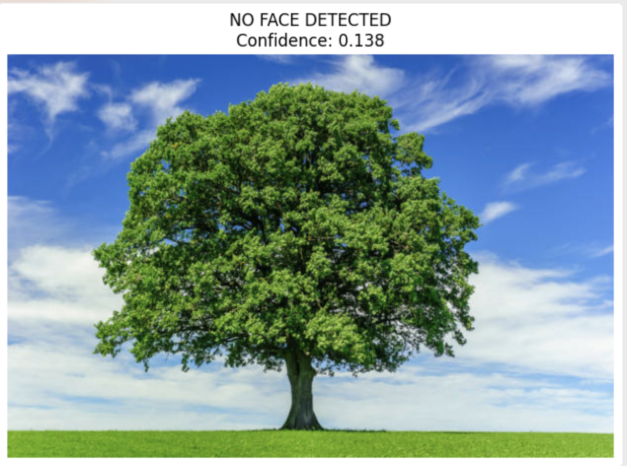
Fig 11. No face detected in picture of tree..
Conclusion
The journey of face detection technologies illustrates a remarkable progression of computational intelligence and machine learning techniques. From Rowley’s pioneering neural network approach in 1998 to the breakthrough Viola-Jones detector in 2001, and culminating in the Deep Dense Face Detector (DDFD), each iteration has systematically addressed the complex challenges of detecting human faces across diverse conditions.
DDFD’s approach demonstrates the power of specialized deep learning architectures. By leveraging a sliding window technique and dense feature abstraction, it achieved superior accuracy while maintaining computational efficiency. Its practical application in face detection and tagging systems, as demonstrated by Mehta et al., underscores the real-world potential of such advanced computer vision techniques.
Looking ahead, the trajectory of face detection suggests continued refinement towards more robust, efficient, and contextually aware systems. Key areas of future development will likely include improving performance on challenging datasets, reducing computational requirements, and addressing potential biases in detection across diverse populations.
References
[1] Farfade, Sachin Sudhakar, Mohammad Saberian, and Li-Jia Li. “Multi-view Face Detection Using Deep Convolutional Neural Networks.” Proceedings of the IEEE/CVF Conference on Computer Vision and Pattern Recognition. 2015.
[2] Rowley, Henry A., Shumeet Baluja, and Takeo Kanade. “Neural Network-Based Face Detection.” IEEE Transactions on Pattern Analysis and Machine Intelligence 20.1 (1998): 23-38.
[3] Girshick, Ross, et al. “Rich feature hierarchies for accurate object detection and semantic segmentation.” CVPR. 2014.
[4] Mehta, Jinesh, Eshaan Ramnani and Sanjay Singh, “Face Detection and Tagging Using Deep Learning.” 2018 International Conference on Computer, Communication, and Signal Processing (ICCCSP), Chennai, India, 2018, pp. 1-6, doi: 10.1109/ICCCSP.2018.8452853.
[5] PuchatekwSzortach. (2024). face_detection. GitHub repository, https://github.com/PuchatekwSzortach/face_detection