Vehicle Trajectory Prediction
This project explores advanced vehicle trajectory prediction methods, a critical component for safe and efficient autonomous driving. By analyzing models like STA-LSTM, Convolutional Social Pooling, and CRAT-Pred, it highlights their unique approaches to handling spatial and temporal complexities, as well as their applications in structured and unstructured traffic environments.
- Introduction
- LSTMs With Spatial–Temporal Attention Mechanisms
- Convolutional Social Pooling Model
- CRAT-Pred
- Comparison of Models
- Reference
Introduction
Motivation
Human drivers are remarkably adept at navigating complex traffic scenarios, drawing on a wealth of perceptual cues and implicit social understanding. Subtle indicators, such as slight speed adjustments, turn signals, and even mutual eye contact, enable them to anticipate the actions of surrounding vehicles, pedestrians, and other road agents. This extraordinary skill underpins safe and efficient driving: it prevents accidents, smooths out congestion, and ensures seamless journeys. Yet, as we envision a future in which autonomous vehicles populate our streets, replicating this human-like forecasting capability poses a profound challenge.
Achieving accurate, reliable vehicle trajectory prediction is central to advancing autonomous transportation. Such predictive models stand to greatly enhance overall safety, reducing human-error-related incidents. They promise to facilitate smoother traffic flow, optimizing road usage and improving travel times for individual drivers and public transportation systems alike. In short, effective trajectory prediction strategies will play a pivotal role in ensuring that autonomy on our roads scales seamlessly from controlled test environments to real-world, dynamic scenarios.
Problem Framework
At its core, trajectory prediction involves forecasting the spatial coordinates of a vehicle over short-term (1–3 seconds) and longer-term (3–5 seconds) horizons. It draws from observed states of the ego vehicle and the myriad agents surrounding it: cars, buses, pedestrians, cyclists, and even animals. By inferring how each participant might move through a shared environment, an autonomous system can proactively adjust its own path to avert collisions and ensure fluid mobility. The challenge is inherently complex, since different agents exhibit diverse and non-linear behaviors that vary across a range of environmental conditions.
Current Challenges
Despite significant progress, vehicle trajectory prediction still faces formidable hurdles. Long-horizon forecasting, for instance, requires extrapolating far into the future (10–20 seconds), where compounding uncertainties can cause small initial differences to yield radically divergent eventual outcomes. Likewise, the underlying driver intentions are non-deterministic and often hidden, making it difficult to formulate a single accurate prediction.
Even more complicated is the need for robustness across heterogeneous scenarios. Models must handle dense urban intersections, rural highways, adverse weather conditions, poor lighting, and fluctuating traffic densities—each scenario demanding resilience and adaptability. Developing predictive frameworks that consistently perform under these broad conditions remains an open and pressing research frontier.
LSTMs With Spatial–Temporal Attention Mechanisms
Lin et al.[3] proposed a state-of-the-art trajectory prediction model that integrates Long Short-Term Memory (LSTM) networks with spatial-temporal attention mechanisms. While traditional LSTMs effectively capture sequential dependencies, they fall short in selectively emphasizing the most critical spatial and temporal features. By leveraging attention mechanisms, the model dynamically prioritizes key spatial-temporal interactions, significantly enhancing both the accuracy and efficiency of trajectory predictions for autonomous systems.
Dataset
The dataset used for training and evaluation is the Next Generation Simulation (NGSIM) dataset, consisting of vehicle trajectory data from segments of U.S. Highway 101 (5 lanes) and Interstate 80 (6 lanes), covering a 2100-foot study area. Each dataset segment contains 45 minutes of data recorded at 10 Hz, divided into three subsets, providing a substantial amount of training and evaluation data. One drawback of it, as mentioned in the paper, is that the dataset only includes forward-moving and lane-changing scenarios, with no additional preprocessing, such as normalization. The image illustrates the study area’s schematic, camera coverage, and a frame from the dataset showcasing labeled vehicle trajectories.
![Visualized NGSIM Dataset[1]](/CS163-Projects-2024Fall/assets/images/team26/ngsim_dataset.png) Fig 1. NGSIM Dataset: Visualized. [1].
Fig 1. NGSIM Dataset: Visualized. [1].
Module Structure
The STA-LSTM model predicts vehicle trajectories by combining temporal and spatial attention mechanisms. The road is divided into a 3x13 grid, where past T-step historical trajectories of vehicles serve as input, and H-step predicted trajectories of the target vehicle are the output. Inputs, represented by past coordinates of the target vehicle, are embedded and processed through an LSTM model to generate hidden states. Temporal attention weights are computed for each hidden state, which are then combined with spatial attention to compute the tensor cell values for the vehicle. This integration captures long-term dependencies effectively, leveraging LSTM’s memory capabilities. Finally, the output is passed through a feedforward layer to generate predictions.
The overall objective function of the STA-LSTM model is given by: \(\min \frac{1}{N_{\text{train}}} \sum_{i=1}^{N_{\text{train}}} \sum_{j=1}^{H} \left( \hat{X}_{i,j} - X_{i,j} \right)^2\)
Temporal Attention Mechanism
The temporal attention mechanism identifies critical historical trajectories to predict the future behavior of target vehicles. It first processes the T-step historical trajectories of a vehicle \(v\), denoted as \(\{X^v_{t-T+1}, ..., X^v_t\}\), and computes the hidden state \(S^v\) for vehicle \(v\) as:
\[S^v = \{h^v_{t-T+1}, ..., h^v_t\}, \quad S^v \in \mathbb{R}^{d \times T}, \quad h^v_j \in \mathbb{R}^d,\]where \(d\) represents the hidden state length.
The temporal attention weights \(A^v\) are calculated using the formula:
\[A^v = \text{softmax}(\text{tanh}(W_\alpha S^v)), \quad A^v \in \mathbb{R}^{1 \times T}, \quad W_\alpha \in \mathbb{R}^{1 \times d}.\]The hidden states \(S^v\) and temporal attention weights \(A^v\) are then combined to compute the temporal attention output for vehicle \(v\) using:
\[H^v = S^v (A^v)^T = \sum_{j=t-T+1}^t \alpha_j^v h_j^v, \quad H^v \in \mathbb{R}^{d \times 1}.\]This mechanism dynamically focuses on the most relevant temporal information for trajectory prediction.
Spatial Attention Mechanism
The spatial attention mechanism ranks neighboring vehicles based on their influence on the target vehicle. It constructs a tensor cell vector \(G\), where:
\[G^n = \begin{cases} H^v_t, & \text{if any vehicle } v \text{ is located at grid cell } n, \\ 0 \in \mathbb{R}^{d \times 1}, & \text{otherwise.} \end{cases}\]The spatial attention weight \(B_t\), associated with all vehicles at the current time frame, is computed as:
\[B_t = \text{softmax}(\text{tanh}(W_\beta G)), \quad B_t \in \mathbb{R}^{1 \times N}, \quad W_\beta \in \mathbb{R}^{1 \times d}.\]The spatial attention weights \(B_t\) and tensor cell vector \(G\) are combined to compute \(V_t\), aggregating all historical information from the target and surrounding vehicles, as:
\[V_t = G_t (B_t)^T = \sum_{n=1}^N \beta_t^n G^n, \quad V_t \in \mathbb{R}^{d \times 1}.\]The resulting \(V_t\) is then passed through a feedforward neural network to predict the H-step trajectory.
Model Performance
The experiment compares the performance of five models using Root Mean Square Error (RMSE) per prediction time step (0.2 seconds). The benchmark models include:
- Physics-based model: A traditional approach without machine learning.
- Naïve LSTM: LSTM without attention weights.
- SA-LSTM: Incorporates spatial attention only.
- CS-LSTM: A state-of-the-art model that will be described later.
- STA-LSTM (Ours): Combines spatial and temporal attention mechanisms.
The results, shown in Table below, indicate that STA-LSTM achieves the smallest RMSE across all prediction steps, demonstrating superior accuracy. Additionally, STA-LSTM requires an average training time of 5 hours.
![Comparison of STA-LSTM Model and Benchmark Models [3]](/CS163-Projects-2024Fall/assets/images/team26/sta_lstm_results.png) Fig 2. Comparison of STA-LSTM Model and Benchmark Models. [3].
Fig 2. Comparison of STA-LSTM Model and Benchmark Models. [3].
Visualizing temporal attention
The temporal attention weight \(A^v\) is computed using:
\[A^v = \text{softmax}(\text{tanh}(W_\alpha S^v)), \quad A^v \in \mathbb{R}^{1 \times T}, \quad W_\alpha \in \mathbb{R}^{1 \times d},\]where \(W_\alpha\) is a learnable weight matrix.
The results, as shown in the figure below, demonstrate that the LSTM model for individual vehicle temporal attention focuses more on the most recent coordinates of the vehicle, while assigning less weight to earlier trajectories. However, due to the memory advantage of LSTMs, earlier trajectories are not completely forgotten, ensuring that the model retains historical information.
![Temporal-Level Attention Weights [3]](/CS163-Projects-2024Fall/assets/images/team26/temporal_attention.png) Fig 3. Temporal-Level Attention Weights. [3].
Fig 3. Temporal-Level Attention Weights. [3].
Visualizing spatial attention
The spatial attention mechanism is demonstrated in two graphs.
The graph below shows the spatial attention weights when the target vehicle \(v\) changes lanes. At each time step, the grid cells containing neighboring vehicles receive varying attention weights. Normally, the grid cell in front of the vehicle receives the highest weight, but during a lane change, the attention shifts to cells on the side of the vehicle. This indicates that the model successfully captures lane-changing behavior.
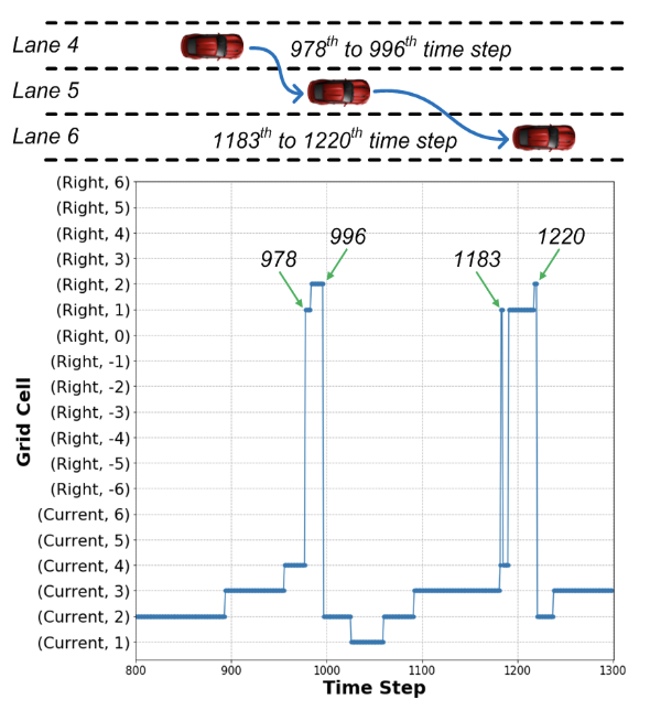 Fig 4. Spatial Attention Weights when Changing Lanes. [3].
The graph below illustrates the density of attention weights across all grid cells. The model focuses primarily on grid cells directly in front of the target vehicle, which is intuitively correct. The absence of attention on cells behind the vehicle (denoted by zeros) confirms that the model focuses on forward-moving vehicles only.
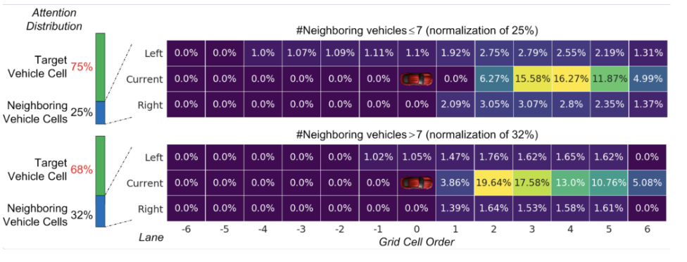 Fig 5. Density of Attention Weights Across All Grid Cells. [3].
Convolutional Social Pooling Model
An alternative approach worth exploring is the method proposed in the paper Convolutional Social Pooling for Vehicle Trajectory Prediction [2]. This method builds on the traditional LSTM-based encoder-decoder framework but introduces innovations to address the spatial interactions among neighboring vehicles with social tensor grids by replacing fully connected layers with a convolutional social pooling layer, allowing the model to maintain spatial locality and better generalize across diverse traffic configurations. Moreover, the maneuver-based decoder enhances multi-modal trajectory prediction by explicitly modeling the probabilities of lateral and longitudinal maneuvers, integrating these probabilities into trajectory generation.
Input and Outputs
For the convolutional social-pooling model, the input to the model is a sequence of past \((x,y)\)-positions of the vehicles for the previous $t_h$ time steps:
\[X = [x(t - t_h), \ldots, x(t - 1), x(t)].\]For each \(x(t)\), we have \((x,y)\) coordinates for the target vehicle and its surrounding vehicles, whose corresponding positions are within $\pm 90$ feet longitudinally and within the two adjacent lanes at each time step:
\[x(t) = [x^{(t)}_0, y^{(t)}_0, x^{(t)}_1, y^{(t)}_1, \ldots, x^{(t)}_n, y^{(t)}_n].\]The outputs of the model are the maneuver class probabilities. Because driver behavior is inherently multi-modal (e.g., a vehicle may continue straight, change lanes left, or change lanes right), we decompose the conditional distribution over a set of maneuver classes \(\{m_i\}\):
\[P(Y \mid X) = \sum_i P(Y \mid m_i, X) P(m_i \mid X).\]Here, \(P(m_i \mid X)\) gives the probability of maneuver class $m_i$, and \(P(Y \mid m_i, X)\) is a bivariate Gaussian distribution parameterized by
\[\Theta = [\Theta(t+1), \ldots, \Theta(t+t_f)],\]corresponding to the means and variances of future locations for that maneuver.
Maneuver Classes
The model considers three lateral maneuvers and two longitudinal maneuvers to capture diverse driving behaviors. The lateral maneuvers include left lane changes, right lane changes, and lane keeping. Recognizing that lane changes require preparation and stabilization, a vehicle is defined as being in a lane-changing state for ±4 seconds relative to the actual cross-over point.
For longitudinal maneuvers, the model distinguishes between normal driving and braking. A braking maneuver is identified when the vehicle’s average speed over the prediction horizon falls below 80\% of its speed at the time of prediction. These maneuver definitions align with how vehicles communicate their intentions through signals, such as turn indicators and brake lights.
![Maneuver Classes [2]](/CS163-Projects-2024Fall/assets/images/team26/maneuver.png) Fig 6. Maneuver Classes. [2].
Fig 6. Maneuver Classes. [2].
Architectural Details
![Convolutional Social Pooling Model Architecture [2]](/CS163-Projects-2024Fall/assets/images/team26/csp_architecture.png) Fig 7. Convolutional Social Pooling Model Architecture. [2].
Fig 7. Convolutional Social Pooling Model Architecture. [2].
LSTM Encoder
The first module encodes the temporal dynamics of each vehicle’s motion. Each vehicle’s past \(t_h\)-frame history is fed into an LSTM encoder:
-
Shared Weights: A single LSTM with shared weights is applied to every vehicle, ensuring a consistent representation across all agents.
-
Vehicle State Encodings: After processing the past \(t_h\) steps, the LSTM’s final hidden state acts as a learned representation of the vehicle’s motion dynamics at time \(t\).
Convolutional Social Pooling
The key challenge is to incorporate information about surrounding vehicles into the prediction for the target vehicle. Previous work used social pooling via fully connected layers or LSTMs to aggregate neighboring vehicle states. However, this approach often fails to leverage the spatial structure of the environment.
Why Convolution Instead of LSTM for Social Pooling?
Traditional LSTM-based social pooling treats all vehicles’ states as elements in a sequence, ignoring the innate spatial relationships. Similarly, fully connected layers do not preserve the neighborhood structure—spatially adjacent cells are treated no differently than distant ones. As a result, if the model never saw a particular spatial configuration in training, it struggles to generalize.
In contrast, applying convolutional layers over a structured “social tensor” preserves and exploits spatial locality. By placing each vehicle’s LSTM-encoded state into a grid cell corresponding to its relative position, we create a spatial map of the scene. Convolutional filters naturally capture local spatial patterns, enabling the model to learn that a vehicle one cell to the left (i.e., one lane over) and slightly behind is more relevant than a distant vehicle multiple cells away. This translational equivariance allows the model to generalize to unseen configurations with greater ease.
Social Tensor Construction
-
Define a \(13 \times 3\) spatial grid around the target vehicle. Each column corresponds to a lane, and each row represents a $\sim 15$-foot segment along the longitudinal axis.
-
Populate the grid with the LSTM states of surrounding vehicles based on their relative positions. Empty cells (no vehicle) can be padded with zeros.
-
Apply two convolutional layers followed by a max-pooling layer to extract a spatial feature encoding. This yields a spatially aware representation—referred to as the \emph{social context encoding}.
Maneuver-Based LSTM Decoder
The decoder takes two components as input: the vehicle dynamics encoding obtained from the target vehicle’s LSTM state after passing it through a fully connected layer, and the social context encoding derived from the convolutional social pooling layers. These encodings are concatenated to form the complete trajectory encoding.
The decoder then outputs probabilities for each maneuver class. Lateral and longitudinal maneuvers are predicted via softmax layers:
\[P(m_i \mid X) = P(\text{lateral maneuver}) \times P(\text{longitudinal maneuver})\]By conditioning on each maneuver class, the decoder produces a maneuver-specific predictive distribution. By concatenating one-hot maneuver indicators with the trajectory encoding, the LSTM-based decoder generates the parameters (\Theta) of the bivariate Gaussian distribution for the future trajectory:
\[P_{\Theta}(Y \mid m_i, X) = \prod_{k=t+1}^{t+t_f}N(y(k) \mid \mu(k), \Sigma(k))\]This formulation allows the model to explicitly represent the multi-modality in future behavior.
Training Details
We train the model end-to-end. Ideally, we would like to minimize the negative log likelihood:
\[-\log \sum_i P_\Theta(Y \mid m_i, X) P(m_i \mid X)\]of the term from Eqn. 5 over all the training data points. However, each training instance only provides the realization of one maneuver class that was actually performed. Thus, we minimize the negative log likelihood:
\[-\log \big(P_\Theta(Y \mid m_{\text{true}}, X) P(m_{\text{true}} \mid X)\big)\]CRAT-Pred
Earlier, the solutions we explore utilize spatial and temporal dynamics but rely heavily on rasterized map data. CRAT-Pred [4] introduces a novel approach to trajectory prediction, leveraging Crystal Graph Convolutional Neural Networks (CGCNNs) and Multi-Head Self-Attention (MHSA) in a map-free, interaction-aware framework.
CRAT-Pred achieves high performance by combining temporal and spatial modeling with efficient graph-based and attention mechanisms. Let’s explore the architecture and methodology in detail.
Architectural Details
![CRAT-Pred Architecture Overview [4]](/CS163-Projects-2024Fall/assets/images/team26/crat_architecture.png) Fig 8. CRAT-Pred Architecture Overview. [4].
Fig 8. CRAT-Pred Architecture Overview. [4].
CRAT-Pred begins by encoding temporal information of vehicle trajectories. Each vehicle’s motion history is represented as a sequence of displacements and visibility flags. The displacement vector \(\Delta \tau_i^t = \tau_i^t - \tau_i^{t-1}\) captures the positional change between successive time steps, and a binary flag \(b_i^t\) indicates whether the vehicle is visible at time \(t\). Together, they form the input representation \(s_i^t = (\Delta \tau_i^t \| b_i^t)\). These inputs are processed by a shared LSTM layer that encodes temporal dependencies for all vehicles. The hidden state of the LSTM, \(h_i^t = \text{LSTM}(h_i^{t-1}, s_i^t; W_{\text{enc}}, b_{\text{enc}})\), summarizes the motion history into a compact, 128-dimensional representation.
The next stage involves modeling spatial interactions between vehicles using a fully connected graph. Each vehicle serves as a node, initialized with its LSTM-encoded hidden state, \(v_i^{(0)} = h_i^0\). Edges in the graph capture pairwise distances between vehicles, defined as \(e_{i,j} = \tau_j^0 - \tau_i^0\). The Crystal Graph Convolutional Network (CGCNN) updates these node features while incorporating edge information. The graph convolution operation is given by \(v_i^{(g+1)} = v_i^{(g)} + \sum_{j \in N(i)} \sigma(z_{i,j}^{(g)} W_f^{(g)} + b_f^{(g)}) \cdot g(z_{i,j}^{(g)} W_s^{(g)} + b_s^{(g)})\), where \(z_{i,j}^{(g)} = [v_i^{(g)} \| v_j^{(g)} \| e_{i,j}]\) is the concatenation of node and edge features. This design allows the model to capture spatial dependencies effectively. Two graph convolution layers are used, each followed by batch normalization and ReLU activations.
To further refine the understanding of interactions, CRAT-Pred applies a multi-head self-attention mechanism. This mechanism computes pairwise attention scores that indicate the influence of one vehicle on another. For each attention head, the output is calculated as \(\text{head}_h = \text{softmax}\left(\frac{V^{(g)} Q_h (V^{(g)} K_h)^\top}{\sqrt{d}}\right) V^{(g)} V_h\), where \(Q_h, K_h,\) and \(V_h\) are linear projections of the node features, and \(d\) is a scaling factor based on the embedding size. Outputs from all heads are concatenated and transformed as \(A = \left[\text{head}_1 \| \dots \| \text{head}_{L_h}\right] W_o + b_o\), resulting in a 128-dimensional interaction-aware embedding for each vehicle. The attention weights provide interpretable measures of interaction strength between vehicles.
The trajectory prediction is performed by a decoder that uses residual connections to refine the output. The decoder predicts positional offsets relative to the initial position of the vehicle, defined as \(o_i = \left(\text{ReLU}\left(F(a_i; \{W_r, b_r\}) + a_i\right)\right) W_{\text{dec}} + b_{\text{dec}}\). Here, \(F(a_i)\) applies non-linear transformations to the interaction-aware features \(a_i\), while the residual connection enhances stability and performance. CRAT-Pred supports multi-modality by using multiple decoders to predict diverse plausible trajectories. These decoders are trained using Winner-Takes-All (WTA) loss, which optimizes only the decoder with the lowest error for each sequence, ensuring diversity in the predictions without complicating the training process.
Training and Evaluation
The training of CRAT-Pred follows a two-stage process. Initially, the model is trained end-to-end with a single decoder using smooth-L1 loss to predict the most probable trajectory. Once this phase converges, additional decoders are introduced, and the model is fine-tuned using WTA loss to handle multi-modal predictions. This approach ensures that CRAT-Pred can produce diverse yet accurate predictions.
CRAT-Pred is evaluated on the Argoverse Motion Forecasting Dataset, which provides large-scale, real-world vehicle trajectory data. The performance metrics include minimum Average Displacement Error (minADE), minimum Final Displacement Error (minFDE), and Miss Rate (MR). These metrics measure the average error of predicted trajectories, the final displacement error, and the percentage of predictions that miss the ground truth by more than 2 meters, respectively. CRAT-Pred achieves state-of-the-art results among map-free models, outperforming many competitors even with significantly fewer model parameters.
![CRAT-Pred Argoverse results [4]](/CS163-Projects-2024Fall/assets/images/team26/crat_results.png) Fig 9. CRAT-Pred Argoverse results. [4].
Fig 9. CRAT-Pred Argoverse results. [4].
The qualitative results of CRAT-Pred on the Argoverse validation set are presented above for three diverse sequences. The past observed trajectory of the target vehicle is depicted in blue, while the ground-truth future trajectory is shown in green. Predicted trajectories are illustrated in orange and red, with orange indicating the most probable future trajectory. The past trajectories of other vehicles are visualized in purple. For context, road topologies, though not utilized by the prediction model, are displayed using dashed lines.
Comparison of Models
The three methods discussed—STA-LSTM, Convolutional Social Pooling, and CRAT-Pred—each present unique strengths and limitations, catering to different aspects of the trajectory prediction problem. STA-LSTM excels in integrating sequential dependencies with spatial-temporal attention, offering an interpretable and computationally efficient approach. However, its reliance on grid-based representations can limit generalizability in highly dynamic, unstructured environments.
The Convolutional Social Pooling model addresses spatial locality effectively by using social tensor grids and convolutional layers. This method is particularly advantageous in scenarios with dense traffic, where spatial relationships among vehicles are critical. Its convolutional layers ensure robustness to diverse traffic configurations, but the model’s performance depends heavily on well-structured input data, such as fixed lane grids, making it less adaptable to unconventional road layouts.
CRAT-Pred, on the other hand, stands out for its map-free framework and advanced graph-based reasoning. By leveraging Crystal Graph Convolutional Neural Networks and multi-head self-attention, it captures both spatial interactions and temporal dynamics without relying on predefined road structures. This flexibility makes CRAT-Pred ideal for real-world applications involving unstructured or rapidly changing environments. However, its complexity and higher computational cost may pose challenges for real-time deployment in resource-constrained systems.
In summary, STA-LSTM offers simplicity and interpretability, making it suitable for grid-based, structured scenarios. Convolutional Social Pooling provides robust spatial handling for dense, structured traffic. CRAT-Pred excels in flexibility and performance in unstructured environments but comes with increased computational demands. The choice of method ultimately depends on the specific requirements and constraints of the autonomous driving application.
Reference
[1] B. Coifman and L. Li, “A critical evaluation of the Next Generation Simulation (NGSIM) vehicle trajectory dataset,” Transportation Research Part B: Methodological, 2017, vol. 105, pp. 362-377, doi: 10.1016/j.trb.2017.09.018.
[2] N. Deo and M. M. Trivedi, “Convolutional Social Pooling for Vehicle Trajectory Prediction,” 2018 IEEE/CVF Conference on Computer Vision and Pattern Recognition Workshops (CVPRW), Salt Lake City, UT, USA, 2018, pp. 1549-15498, doi: 10.1109/CVPRW.2018.00196.
[3] L. Lin, W. Li, H. Bi and L. Qin, “Vehicle Trajectory Prediction Using LSTMs With Spatial–Temporal Attention Mechanisms,” in IEEE Intelligent Transportation Systems Magazine, vol. 14, no. 2, pp. 197-208, March-April 2022, doi: 10.1109/MITS.2021.3049404.
[4] J. Schmidt, J. Jordan, F. Gritschneder and K. Dietmayer, “CRAT-Pred: Vehicle Trajectory Prediction with Crystal Graph Convolutional Neural Networks and Multi-Head Self-Attention,” 2022 International Conference on Robotics and Automation (ICRA), Philadelphia, PA, USA, 2022, pp. 7799-7805, doi: 10.1109/ICRA46639.2022.9811637.