Text-To-Image Generation - A Study of CV Models Shaping the Newest Tool in Creative Expression
The goal of this study is to analyze different approaches to text to image generation. We specifically looked at innovations being made with GANs and diffusion models. This study explores the implementations of StackGAN, latent diffusion models, and Stable Diffusion XL (SDXL).
1. Introduction
The ability to generate high-quality, meaningful images from textual descriptions has emerged as one of the most exciting advancements in the intersection of artificial intelligence and computer vision. Text-to-image generation models leverage natural language processing (NLP) and deep learning to create visual representations of written descriptions, enabling machines to bridge the gap between text and visual understanding. These models hold the promise of transforming industries ranging from entertainment and design to education and accessibility.
Early attempts in this field were limited by the challenges of understanding complex textual prompts and generating coherent, high-resolution images. However, recent innovations, such as the integration of transformer architectures, diffusion models, and large-scale pretraining, have dramatically improved the quality and fidelity of generated images. Models like OpenAI’s DALL·E, Google’s Imagen, and Stability AI’s Stable Diffusion have demonstrated an unprecedented ability to produce photorealistic and semantically accurate images, even from nuanced or creative prompts.
This comparative study looks at the current state of text-to-image generation, focusing on the approaches different computer vision models use to achieve high performance and quality results. The three models we will focus on are StackGAN, latent diffusion models, and Stable Diffusion XL (SDXL). By delving into the mechanics and implications of these models, this study aims to provide an understanding of their potential and limitations in shaping the future of AI-driven creativity and content generation.
2. Technical Background
For this study, we first look at two major computer vision models used in text-to-image generation: generative adversarial networks (GAN) and diffusion models.
2.1. GANs
General adversarial networks were one of the major approaches in text-to-image generation in recent years. Figure 1 below lays out generally how a GAN works. The primary training mechanism within a GAN is twofold: a generator, which captures the distribution of true examples of the input sample and generates realistic images, and a discriminator, which classifies generated images as fake and the real images from the original sample as real.
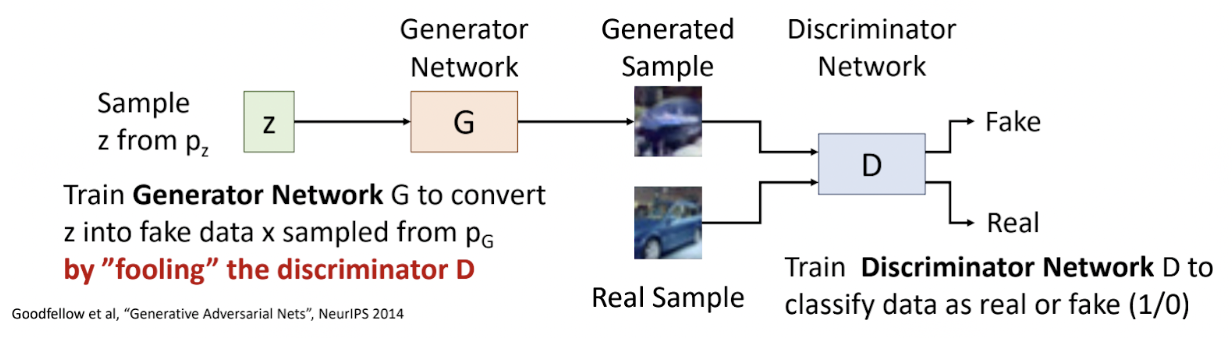
Fig. 1: Image showing basic layout of GAN [5].
The GAN model attempts to optimize and balance the generator’s ability to create realistic images and the discriminator’s ability to differentiate between real and generated images. The generator and discriminator are jointly trained with a minimax game using alternating gradient updates (Figure 2). The minimax game reaches its global minimum (the ultimate goal) when the generated sample converges to the real sample. To train, a minibatch of training points is sampled from the distribution and a minibatch of noise vectors is sampled from p(z). The generator parameters are updated via stochastic gradient descent, while the discriminator parameters are updated via stochastic gradient ascent. After being fed hundreds or thousands of training images, the algorithm outputs a series of generated images in a best-attempt imitation.
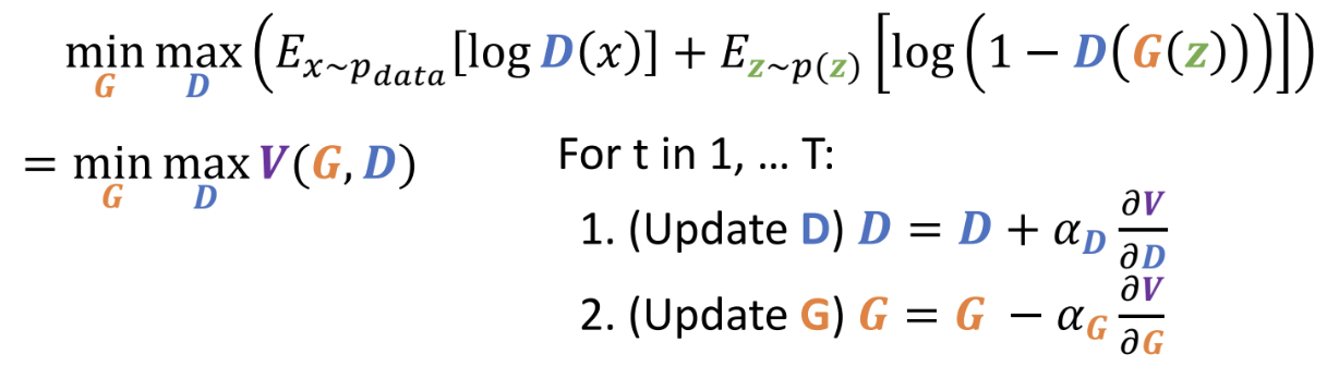
Fig. 2: GAN training equations [5].
2.2. Diffusion Models
Both Latent Diffusion Models and Stable Diffusion XL (SDXL), which are two of the three models discussed later in this report, are both derived from the general diffusion model framework. The diffusion model is a generative model that can be broken down into two parts. The first part, called the forward process, involves adding noise sampled from a Gaussian distribution to an input image over multiple time steps until the image is only noise. Each time step of the forward process can be described using the equations below:
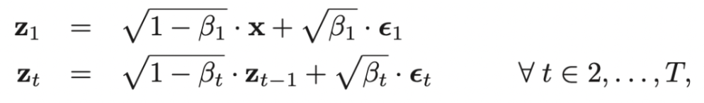
Fig. 3: Equations for forward process of diffusion [5].
\(x\) is the initial input image, \(\epsilon_t\) is noise sampled from a Gaussian distribution at time step \(t\), \(z_t\) is the output at time step \(t\) after applying noise, and \(\beta_t\) is an element from the noise schedule \(\beta\), which influences how much noise is applied to the current image at each time step. As can be observed from the equation, each time step involves combining the output image from the previous time step with some noise.
In the second part, known as the reverse process, the noisy image is processed for several time steps, with each time step removing some of the noise from the image. At the end of the reverse process, the output is a fully denoised image. During training, both the first and second parts are performed to train the diffusion model on a dataset of images. Afterwards, only the second part of the model can be utilized to derive newly generated images from pure noise.
Diffusion models are often implemented using a U-Net (UNet) architecture, which involves downsampling and then upsampling the image. The current iteration of the image is passed through the UNet for each time step to add noise.
Diffusion models are trained to minimize the following loss function.
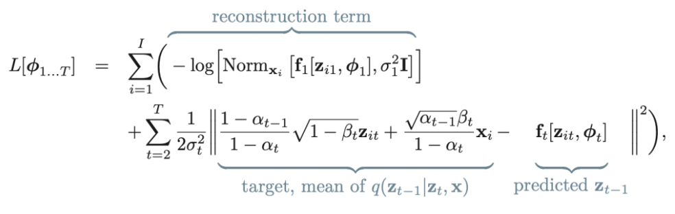
Fig. 4: Loss function for diffusion model [2].
In the loss function shown in Figure 4, \(\phi_t\) represents parameters, \(x_i\) represents an image to train on, \(z_{it}\) represents the latent output at time step \(t\) for the corresponding image, \(\beta_t\) represents an element from the noise schedule, \(\alpha_t\) is given by the result of \(\prod_{s=1}^t {1 - \beta_s}\), \(\sigma_t\) represents some predefined value, and \(f_t\) represents a “neural network that computes the mean of the normal distribution in the estimated mapping from \(z_t\) to the preceding latent variable \(z_{t-1}\)” [2]. As shown in the loss function in Figure 4, the first summation considers the “reconstruction term” [2]. More notably, the second summation corresponds to minimizing the difference between the image in the forward process and in the reverse process at a given time step.
3. Model Analysis
3.1. Specific Implementations
3.1.1. StackGAN
The first model considered in this study is Stacked General Adversarial Networks, or StackGAN. This model attempts to address the challenge of producing high-resolution images by decomposing the generation process into two stages, each handled by a dedicated GAN. This staged approach is intended to improve image quality and ensure that finer details align with textual input.
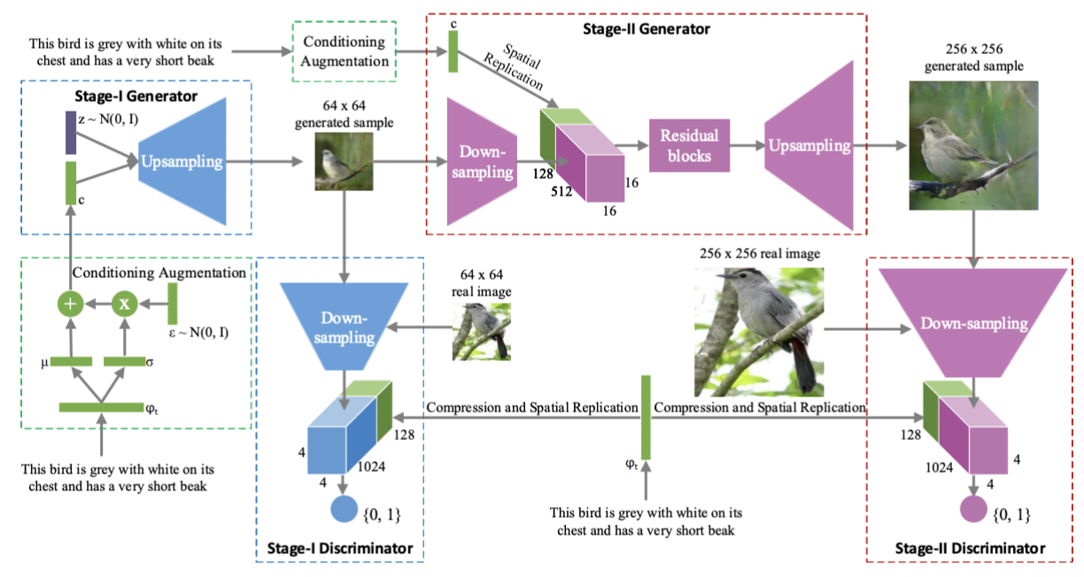
Fig. 5: Diagram of overall StackGAN structure [4].
The Stage-I GAN is designed to create a low-resolution (64×64) image that captures the basic structure and colors described in the input text. It employs a text encoder to extract semantic embeddings, which are augmented through a conditioning technique that samples latent variables from a Gaussian distribution creating a conditioning vector. This augmentation smoothens the manifold – a mathematical concept detailing a high-dimensional space where data points lie on a lower-dimensional structure. This improves robustness and generates diverse outputs. As laid out in Figure 5, the Stage-I generator takes in that textual embedding, and conditioning vector concatenated with a noise vector (z ~ N(0,1)). The concatenated vector passes through an upsampling network to generate a coarse, low-resolution image (64×64). This image captures the basic layout, colors, and structure based on the textual description. The images produced by the Stage-I generator are often coarse, lacking intricate details and sometimes distorted. The Stage-I discriminator receives either the real 64×64 image or the generated image, along with the text embedding, downsamples and compresses the image while the text embedding is spatially replicated to align with the image features, and then predicts whether the input image is real or fake and checks if it matches the text description.
Building on the Stage-I output, the Stage-II GAN refines the image to produce a high-resolution (256×256) version with vivid details. It corrects defects in the initial image while reprocessing the text embedding to incorporate overlooked information. Using residual blocks for feature refinement and up-sampling layers to enhance resolution, Stage-II ensures the generated images are realistic and textually accurate. As seen in Figure 3, the Stage-II generator takes in the low-resolution (64×64) image from Stage-I and the original text embedding. The 64×64 image is downsampled, and the text embedding is spatially replicated. These inputs are passed through several residual blocks to refine features and enhance details, correcting any artifacts from Stage-I. The refined features are then passed through upsampling layers to generate a high-resolution (256×256) image. The Stage-II discriminator receives either the real 256×256 image or the generated image, along with the text embedding. The input image is downsampled, and the text embedding is spatially replicated and compressed. The discriminator determines whether the input image is real or fake and verifies alignment with the text description. By conditioning on both the low-resolution image and the original text, this stage efficiently captures and enhances fine-grained details.
The training process for both GANs incorporates adversarial loss to encourage realistic image synthesis, conditional loss to align images with textual descriptions, and Kullback-Leibler divergence to regularize the latent space. The architecture ensures a smooth progression from coarse sketches to detailed images, yielding outputs that significantly outperform prior methods.
3.1.2. Latent Diffusion Models
The next model considered in this study is latent diffusion. Latent diffusion models (LDMs) represent a significant advancement in high-resolution image synthesis by introducing the concept of working within a compressed latent space, rather than pixel space, which reduces computational costs while preserving the quality of the generated images. This makes it possible to generate detailed, high-quality images without taking up excessive computational overhead. The model’s architecture uses a pre-trained autoencoder to map images to a lower-dimensional latent representation, where the diffusion takes place. The decoder reconstructs these latent representations back into the pixel space, ensuring the generated outputs have a high fidelity. The figure below, sourced from the paper, shows in more detail how the autoencoder enables the transition between pixel and latent space, capturing both the structural and semantic representations of the input.
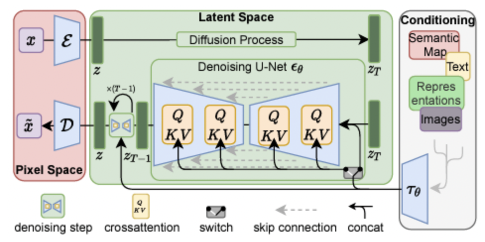
Fig. 6: Representation of LDM Framework [3].
Figure 6 shows a comprehensive representation of the LDM framework, showing how the three main components (the autoencoder, the diffusion model, and the decoder) work together. The autoencoder module compresses the input into latent representations, capturing the essential features, while discarding any unnecessary high-dimensional data. The encoder reduces the complexity of the image, ensuring efficient training and inference. Operating in the latent space, the module performs the core generative process. A series of denoising steps progressively removes noise added during the forward diffusion process, guided by text conditioning through cross-attention mechanisms. The cross-attention layer ensures the alignment of text embeddings with the evolving latent representation. After the denoising process is complete, the decoder reconstructs the latent representation back into pixel space, producing the final high-resolution image. The interplay between all these components ensures the outputs are both photo-realistic and semantically aligned with the text inputs.
The training pipeline consists of two major states: pre-training the autoencoder and training the latent diffusion process. With pre-training the autoencoder, the autoencoder is trained using large-scale datasets like ImageNet to encode and decode images efficiently. The reconstruction loss ensures minimal degradation when converting between pixel and latent spaces. With training the latent diffusion process, the core of the LDM framework involves training the diffusion model to operate within the latent space. The key objective function used for training is the variational lower bound (VLB), which can be decomposed into two main components: reconstruction loss, which ensures the autoencoder accurately reconstructs images from the latent space, preserving structural and semantic details, and denoising score-matching loss, which trains the diffusion process to iteratively remove noise from corrupted latent representations. This loss encourages the model to generate realistic latent representations that align with the text inputs, ensuring high fidelity and semantic relevance in the final images.
3.1.3. SDXL (Stable Diffusion XL)
The last model to be discussed is Stable Diffusion XL, or SDXL for short. SDXL evolved from Stable Diffusion, which is based on latent diffusion models and has a specialized focus on text-to-image generation. The goal of SDXL was to significantly improve the performance of previous latent diffusion models in terms of the quality of images generated, as well as resolve notable problems with Stable Diffusion. SDXL’s improved performance was achieved through three significant changes and additions: an improved UNet architecture for the backbone of the model, two conditioning techniques, and a refinement model. These three changes are described in more depth below.
The first major change involved modifying the structure of the UNet backbone. SDXL still utilizes cross-attention like how it was used in latent diffusion models. Beyond this similarity, modifications to the UNet are summarized in the table below.
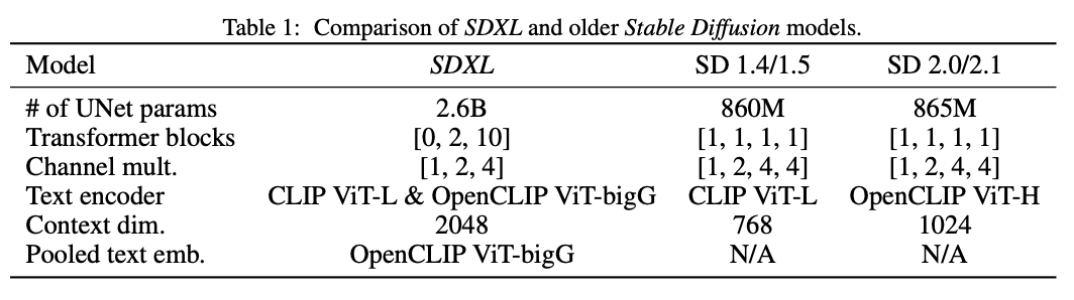
Fig. 7: Architecture of SDXL and SD versions [1].
As can be observed from the table in Figure 7, one notable change is the number of levels in the UNet. Instead of having four levels, the UNet in SDXL has only three levels and forgoes the level that downsamples the image by a factor of 8. Another change was the placement of transformer blocks throughout the UNet architecture. Instead of a single transformer block at each of the four levels of the UNet (as in Stable Diffusion), there are 0, 2, and 10 transformer blocks at the 1st, 2nd, and 3rd highest levels of the UNet respectively. SDXL also uses the joined outputs of two text encoders, CLIP ViT-L and OpenCLIP ViT-bigG, instead of one in order to elevate the performance in regards to conditioning on text inputs. These modifications significantly increased the number of parameters in the UNet, resulting in a total of 2.6 billion parameters.
The second change involves the use of conditioning mechanisms, which were specifically added to address the problem with how latent diffusion models have a limit on the smallest size that images can be for training. This is an important limitation to resolve as removing this limitation will allow for training on larger sets of data that include such smaller images. SDXL, therefore, also conditions on the size of the training image, given as \(c_{size} = (h_{original}, w_{original})\). By adding this additional condition, the model is able to additionally learn the correlation between image sizes and the quality (or resolution) of visual features. Therefore, this enables flexibility in controlling the quality of image generation, as the “apparent resolution” [1] can be specified to the model. As can be observed in the diagram below (Figure 8), specifying higher resolutions for the generated image creates more distinct visual features.
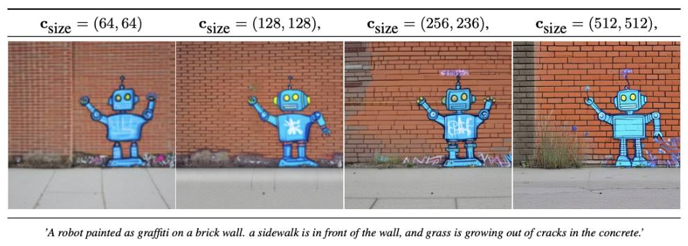
Fig. 8: Images generated by SDXL, using different size conditions [1].
Another conditioning mechanism that was added for SDXL was controlling the degree of cropping for generated images. Due to the use of random cropping in the data augmentation step of training Stable Diffusion, the generated images from Stable Diffusion would crop the desired objects. To resolve this, SDXL requires the specification of \(c_{top}\) and \(c_{left}\) for images during training, which collectively indicate the number of pixels by which the top and left sides of the image were cropped. These two values can then be specified when using the model, allowing for more flexibility to control the degree of cropping in the generated images.
Both conditioning mechanisms for resolution and cropping are passed into the UNet of SDXL as combined feature embeddings.
The final major change made when developing SDXL was the addition of a refinement model. The goal of the refinement model is to further enhance the quality of SDXL’s generated images. The refinement model also uses a latent diffusion model as a base, and removes the noise from the latent outputs of the base SDXL model. Despite improved quality in generated images, it is important to note that the use of two latent diffusion based models for SDXL is more expensive both in terms of memory and computation. The architecture of the final SDXL model is shown in the image below (Figure 9).
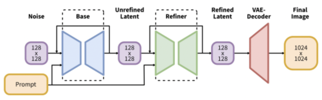
Fig. 9: Diagram of SDXL model structure [1].
3.2. Performance Comparisons
3.2.1. StackGAN Performance
The hierarchical nature of StackGAN’s architecture is a key factor in its success. By breaking down the generation process into two stages, StackGAN simplifies the task of what is often a highly computationally expensive process of high-resolution image synthesis. Stage-I focuses on producing a coarse but textually accurate representation, while Stage-II specializes in enhancing details and overall image quality. This staged approach allows StackGAN to generate images that are significantly more realistic and aligned with textual descriptions compared to single-stage methods. Evaluations on datasets such as CUB (birds) and Oxford-102 (flowers) demonstrate StackGAN’s effectiveness, as it achieves higher inception scores and better human ratings than earlier approaches like GAN-INT-CLS and GAWWN (Figure 10 and 11). For the CUB dataset, the 64×64 samples generated by GAN-INT-CLS can only reflect the general shape and color of the birds. The images don’t have vivid parts (e.g., beak and legs) and convincing details in most cases, which make them neither realistic enough nor sufficiently high resolution. With additional conditioning variables on location constraints, GAWWN obtains a better inception score, but StackGAN still easily outperforms both approaches.
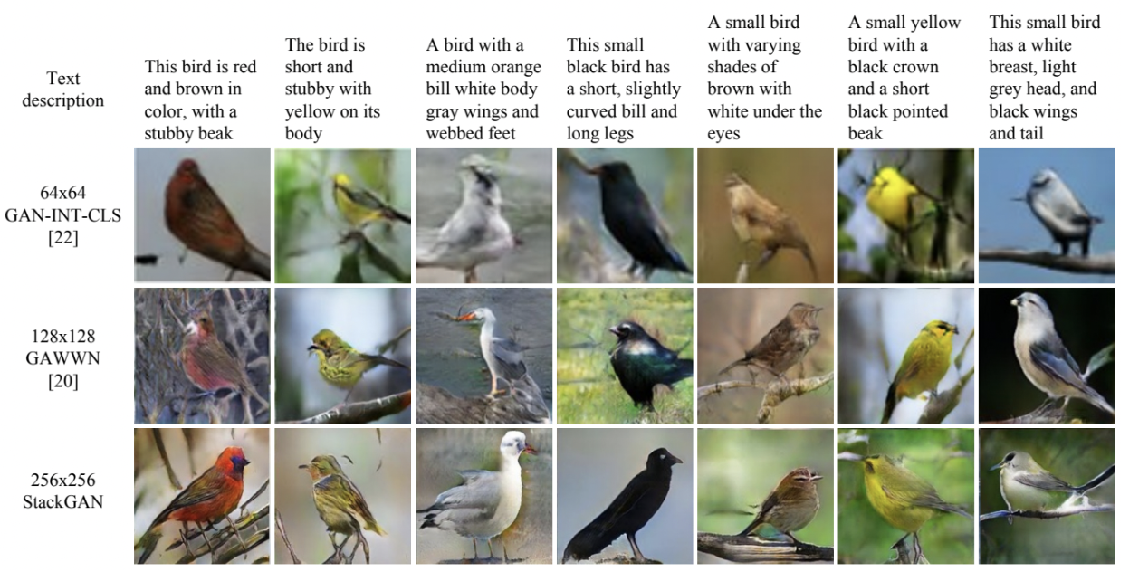
Fig. 10: CUB dataset comparative results between StackGAN and other GANs [4].
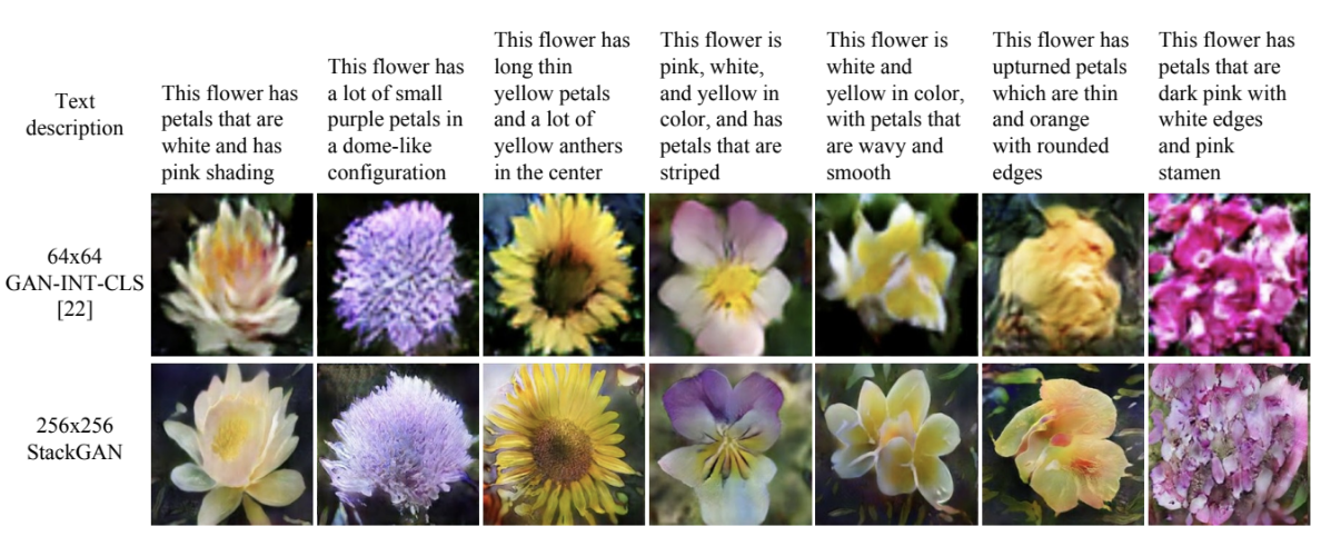
Fig. 11: Oxford-102 dataset comparative results between StackGAN and other GANs [4].
StackGAN excels in generating realistic, high-resolution images from textual descriptions by decomposing the synthesis task into manageable subtasks. Its innovative conditioning mechanisms, hierarchical design, and use of adversarial training contribute to its superior performance. These features make StackGAN a groundbreaking model in text-to-image synthesis, with potential applications in fields like design, content creation, and synthetic data generation.
3.2.2 Latent Diffusion Performance
Latent diffusion models (LDMs) achieve significant advancements in generating high-resolution, photo-realistic images with computational efficiency. Evaluations presented in the paper demonstrate LDMs outperform pixel-space diffusion models on key benchmarks, including FID (Frechet Inception Distance), CLIP consistency, and efficiency gains. For FID, the LDM framework yields lower FID scores compared to prior approaches, indicating its ability to generate more realistic and visually coherent images. In particular, the paper highlights improvements when evaluated on datasets like MS-COCO and ImageNet, achieving state of the art performance. For CLIP consistency, by leveraging cross-attention mechanisms during the diffusion process, LDMs maintain strong alignment between the generated images and the provided text descriptions. This alignment is quantitatively measured using CLIP scores, where LDMs surpass competing methods such as DALL·E and stable diffusion. For efficiency gains, operating in a compressed latent space reduces the model’s memory and computational requirements. The paper notes that LDMs achieve similar or superior visual quality with only a fraction of the computational resources required by pixel-space diffusion models.
When benchmarked against alternative frameworks, such as GAN-based and pixel-space diffusion models, LDMs consistently demonstrate superior scalability and text-image fidelity. For superior scalability, the use of latent representations enables the generation of 1024x1024 or higher resolution images without prohibitive computational costs. For text-image fidelity, qualitative comparisons reveal that LDMs better align with textual prompts. However, LDMs also have limitations, such as dependence on autoencoder quality and training complexity. For dependence on autoencoder quality, the fidelity of the latent representation heavily relies on the pre-trained autoencoder. Any loss in information during encoding can affect the quality of generated images. For training complexity, the two-stage training process (autoencoder pretraining and latent diffusion training) adds complexity and increases overall training time compared to single-stage methods.
3.2.3. SDXL Performance
SDXL significantly enhances the performance of latent diffusion models, particularly in high resolution text to image synthesis. The paper presents key improvements in quantitative metrics, such as FID (Frechet Inception Distance) and IS (Inception Score). For FID, SDXL achieves improved FID scores compared to earlier versions of stable diffusion (1.5 and 2.1), indicating better image realism. For example, on class-conditional ImageNet, conditioning the model on spatial size reduced FID from 43.84 (non-conditioned) to 36.53, showcasing the impact of enhanced conditioning techniques. For IS, the introduction of additional conditioning on input size and cropping parameters boosts the Inception Score, improving semantic alignment and visual coherence. The IS for size-conditioned models increased to 215.50, reflecting superior image quality and detail.
Improvements over previous models include the expanded UNet backbone, novel conditioning techniques, and post-hoc refinement model. SDXL uses a UNet architecture with triple the attention blocks and a second text encoder, significantly increasing its capacity for capturing detailed representations. This larger architecture supports higher resolution outputs with fewer artifacts. SDXL uses novel conditioning techniques, such as size and crop conditioning during training, which reduces artifacts and improves the alignment of generated content with input prompts. This method addresses challenges like random cropping during training, which previously led to inconsistent results. For the post-hoc refinement model, a refinement step further enhances the quality of generated images by removing residual noise from the latent representations. This process ensures sharper and more detailed outputs while maintaining efficiency.
4. Conclusion
When trying to determine which model to use, the most important contributing factor is the ultimate end goal of the user. StackGAN is ideal for simpler text-to-image synthesis, as its hierarchical stages help produce extremely realistic results at the cost of limited scalability. Latent Diffusion Models (LDMs) excel at producing results with computational efficiency while remaining true to the initial text prompt, but are limited by their reliance on autoencoders and complex training. Stable Diffusion XL (SDXL) further adds to the existing LDM techniques, addressing several of LDM’s pitfalls along the way.
StackGAN’s simplified stage structure allows the model to better enhance details and create stronger alignment to the text prompt of the user, but its scalability is limited to very high resolutions (e.g. 1024 x 1024). LDMs’ use of compressed latent space encodings reduces memory overhead and computational costs, leading to superior scalability and text-image fidelity compared to GAN-based models like StackGAN. However, LDMs’ heavy reliance on the quality of the pre-trained autoencoder and two-stage training complicates training and adds to training time. Stable Diffusion XL (SDXL) is more advanced compared to LDMs, providing more flexibility, refined conditioning, and higher resolution to generated images. However, SDXL is more computational and memory heavy compared to LDMs due to their two part structure (a base latent diffusion based model and a refinement latent diffusion based model). SDXL is able to create high resolution outputs like StackGAN is but with a minimization of visual irregularities and imperfections in the generated image through conditioning and a final processing step to enhance resolution and image quality. While StackGAN carries limitations in resolution and scalability, SDXL is primarily limited by available computational resources, which it requires more of compared to other LDMs and prior models.
Depending on the available computational resources, training time, and specific project needs, any of these models is capable of producing high-quality, high-resolution images in alignment with the initial user text prompt.
5. References
[1] Podell, Dustin, et al. “SDXL: Improving Latent Diffusion Models for High-Resolution Image Synthesis.” arXiv preprint arXiv:2307.01952, 2023. (https://arxiv.org/abs/2307.01952)
[2] Prince, Simon J.D. “Understanding Deep Learning.” The MIT Press, 2024. (https://udlbook.github.io/udlbook/)
[3] Rombach, Robin, et al. “High-Resolution Image Synthesis with Latent Diffusion Models.” Proceedings of the IEEE/CVF Conference on Computer Vision and Pattern Recognition, 2022. (https://arxiv.org/pdf/2112.10752)
[4] Zhang, Han, et al. “StackGAN: Text to Photo-Realistic Image Synthesis with Stacked Generative Adversarial Networks.” ICCV, 2017. (https://arxiv.org/pdf/1612.03242v1)
[5] Zhou, Bolei. “Lecture 16: Generative Models: VQ-VAE, GANs, and Diffusion Models.” UCLA COM SCI 163: Deep Learning for Computer Vision, 2024.