Anti-Facial Recognition Technology
In this article, we examine various anti-facial recognition techniques and assess their effectiveness. We begin by introducing facial recognition and providing a high-level overview of its pipeline. Next, we explore how Fawkes software exploits vulnerabilities in image cloaking by testing it on the PubFig database. We then discuss MTCNN-Attack, which prevents models from recognizing facial features by overlaying grayscale patches on individuals’ faces. Finally, we present a method that adds noise to images, rendering them unlearnable to models while remaining visually indistinguishable to the naked eye.
Introduction
Facial Recognition (FR) systems are designed to identify individuals by analyzing and comparing their facial characteristics. Unlike facial verification systems, which primarily authenticate users on devices (such as Apple’s FaceID by matching a user’s face to a single stored feature vector), FR systems focus on recognizing individuals from a larger pool of known identities.
However, as facial recognition technology becomes increasingly integrated into daily life, privacy and security concerns have emerged. This has led to the development of anti-facial recognition (AFR) tools that strategically target vulnerabilities in the FR pipeline to prevent accurate identification of individuals.
FR Pipeline
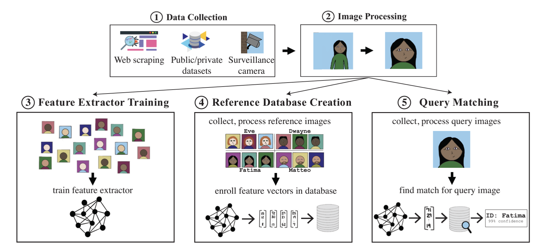
Fig. 1. Division of the facial recognition pipeline into 5 stages. Taken from [4]
The operational workflow of FR systems can be divided into five critical stages:
- Image Collection: FR systems gather face images from various sources, including online scraping or capturing photos directly. This stage is foundational, as the quality and diversity of collected images significantly impact the system’s effectiveness.
- Image Preprocessing: Preprocessing involves detecting and cropping faces from images, followed by normalizing the data to ensure uniformity. This step enhances the quality of the input data, making it suitable for accurate feature extraction.
- Training Feature Extractor: Typically a deep neural network (DNN) trained to convert face images into mathematical feature vectors. These vectors are designed to be similar for images of the same person and distinct for different individuals. Training requires vast amounts of labeled data and computational resources.
- Reference Database Creation: Creating a reference database involves storing feature vectors alongside corresponding identities, enabling the system to compare and identify faces accurately. The database must be extensive and well-organized to facilitate quick and reliable matching during the recognition process.
- Query Matching: In real-time operation, the FR system processes an unidentified face image by extracting its feature vector and comparing it against the reference database. Using distance metrics like L2 or cosine similarity, the system identifies the closest match and retrieves the associated identity if the similarity
AFR tools strategically target one or more of the five stages in the FR pipeline to prevent accurate identification of individuals, such as Fawkes acting on the fourth stage and Unlearnable Examples on the third.
Fawkes
Motivation
Facial Recognition poses a serious threat to personal privacy in the modern era of surveillance. Privately owned companies like Clearview.ai scrape billions of images from social media to create a model capable of recognizing millions of citizens without their consent. In general, anti facial recognition technology takes the approach of what is known as a poisoning attack in machine learning, making someone’s face difficult to recognize.
Past attempts include wearables, like glasses or a hat with stickers, which aim to make a person harder to identify. However, these wearables suffer from being clunky, unfashionable, and impractical for daily use. Furthermore, they require full knowledge of the facial recognition system they aim to deceive, which is an unrealistic assumption in the wild. Other attempts use machine learning to edit facial images through use of a GAN or k-means averaging, but these methods alter the content of the image extensively, making them unfit to be used when sharing images on social media.
The Fawkes software targets the third stage of the FR pipeline, aiming to cloak facial images without dramatically altering their appearance. If these cloaked images are shared online and scraped for a facial recognition database, the poisoned image would provide the embedding for face verification. When a clean image is captured in the wild through surveillance technology, it would not find a match in the database as the poisoned embedding is effectively dissimilar to the unaltered facial embedding. The flow of this system is demonstrated in Figure 1.
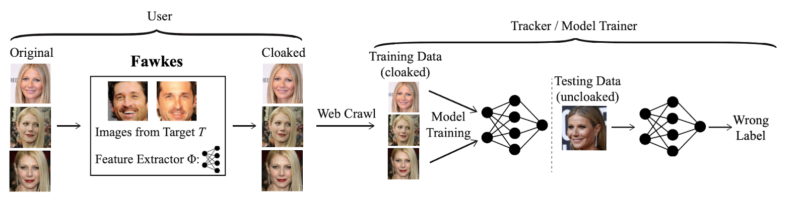 Fig 2. The Fawkes system aims to disrupt facial recognition by poisoning the training database. [1]
Some challenges to this technology are as follows:
- Image labels remain the same during the poisoning process, as they are posted to a known account, so the scope of the attack is limited to editing image contents
- The cloak should be imperceptible, meaning the use of the image for human eyes is not negatively impacted.
- The cloak should work regardless of facial detection model architecture.
Optimizing Cloak Perturbations
The generation of a cloak for a given image can be imagined as a constrained optimization problem, where C is the cloaking function, “Model” is the feature extractor used by the model, x is the original image, x_T is the target image and x ⊕ C(x,x_T) is the cloaked image.
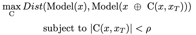
Here, rho is the amount that we are allowing the image to be deviated by. When the real model used by facial recognition technology differs from the model used in cloaking optimization, Fawkes relies on the transferability effect, the property that models trained for similar tasks share similar properties, such as the facial vector embedding.
We can convert the optimization problem into this form:

where taking lambda to infinity would make the image visually identical to the original image by heavily penalizing a cloaking distance larger than rho. This loss function uses the DSSIM (Structural Dis-Similarity Index) to determine if the cloak has overtaken rho in magnitude. Previous work has deemed DSSIM a useful metric at measuring user-perceived image distortion, an unexpected quality of feature vectors extracted by deep learning.
Results
Figure 3 shows a visualization of the effectiveness of cloaking when training on poisoned images.
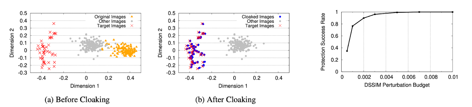 Fig 3. Shown is a plot of embedding vectors after principal component analysis with the impact of cloaking demonstrated in (b). [1]
When training the cloak on a known feature extractor the Fawkes method achieved 100% accuracy when rho, the perturbation margin, is allowed to be greater than 0.005 which is barely detectable to the human eye. As demonstrated in the figure, the cloak is highly effective at changing the representation of the feature vector. However, it is not alway possible to know the feature extraction method of the target model. By using robust feature extractors, models that are trained adversarially to decrease sensitivity to input perturbations can be used as global feature extractors to train the cloaking to work against an unknown model. Using this method, Fawkes is able to achieve a protection success rate greater than 95%. When tested on Microsoft Azure Face API, Amazon Rekognition Face Verification, and Face++, the robust model is able to achieve 100% protection against all three.
Evaluating Fawkes on PubFig
First, I download the pubfig face database from kaggle for use as a dataset.
# installing pubfaces
import kagglehub

# Download latest version
path = kagglehub.dataset_download("kaustubhchaudhari/pubfig-dataset-256x256-jpg")

print("Path to dataset files:", path)
Warning: Looks like you're using an outdated `kagglehub` version, please consider updating (latest version: 0.3.5)
Downloading from https://www.kaggle.com/api/v1/datasets/download/kaustubhchaudhari/pubfig-dataset-256x256-jpg?dataset_version_number=1...


100%|██████████| 176M/176M [00:03<00:00, 50.9MB/s]

Extracting files...


Path to dataset files: /root/.cache/kagglehub/datasets/kaustubhchaudhari/pubfig-dataset-256x256-jpg/versions/1
I installed the deepface repository for facial detection, which comes with a variety of models to use, including VGG-Face, Facenet, OpenFace and DeepFace.
pip install deepface
from deepface import DeepFace
24-12-14 01:21:24 - Directory /root/.deepface has been created
24-12-14 01:21:24 - Directory /root/.deepface/weights has been created
from google.colab import files
For reference, two images of the same person (Bolei Zhou in this case) will generate a distance score of around 0.2 to .4 if taken from a similar angle with similar lighting.
result = DeepFace.verify(
    img1_path = 'images?q=tbn:ANd9GcSYXqI16ROGe18ZVawkpYLCGnqG76Td7WTMRw',
    img2_path = 'prof_pic.jpg'
)
24-12-04 00:24:31 - vgg_face_weights.h5 will be downloaded...


Downloading...
From: https://github.com/serengil/deepface_models/releases/download/v1.0/vgg_face_weights.h5
To: /root/.deepface/weights/vgg_face_weights.h5
100%|██████████| 580M/580M [00:06<00:00, 84.1MB/s]
print(result)
{'verified': True, 'distance': 0.36161117870795056, 'threshold': 0.68, 'model': 'VGG-Face', 'detector_backend': 'opencv', 'similarity_metric': 'cosine', 'facial_areas': {'img1': {'x': 65, 'y': 40, 'w': 84, 'h': 84, 'left_eye': (122, 72), 'right_eye': (90, 72)}, 'img2': {'x': 229, 'y': 140, 'w': 440, 'h': 440, 'left_eye': (523, 321), 'right_eye': (366, 321)}}, 'time': 14.65}
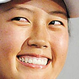
On my personal computer I downloaded the fawkes model and applied it to a picture of our professor, Bolei Zhou.
fawkes_bolei = files.upload()
Saving prof_pic_cloaked.png to prof_pic_cloaked.png
For reference, here is the original image:

And here is the cloaked image:

I also download a different, uncloaked picture which I will use for face identification against the picture.
! wget -O Bolei_Zhou.png https://iu35-prod.s3.amazonaws.com/images/Bolei_Zhou_1.width-3000.png
--2024-12-14 01:21:41--  https://iu35-prod.s3.amazonaws.com/images/Bolei_Zhou_1.width-3000.png
Resolving iu35-prod.s3.amazonaws.com (iu35-prod.s3.amazonaws.com)... 16.15.179.28, 52.217.200.129, 3.5.27.183, ...
Connecting to iu35-prod.s3.amazonaws.com (iu35-prod.s3.amazonaws.com)|16.15.179.28|:443... connected.
HTTP request sent, awaiting response... 200 OK
Length: 2759019 (2.6M) [image/png]
Saving to: ‘Bolei_Zhou.png’

Bolei_Zhou.png      100%[===================>]   2.63M  6.00MB/s    in 0.4s

2024-12-14 01:21:42 (6.00 MB/s) - ‘Bolei_Zhou.png’ saved [2759019/2759019]
I insert the cloaked version of professor Bolei’s face into the directory to be picked up by the database.
! mkdir /root/.cache/kagglehub/datasets/kaustubhchaudhari/pubfig-dataset-256x256-jpg/versions/1/CelebDataProcessed/'Bolei Zhou'/
! mv prof_pic_cloaked.png /root/.cache/kagglehub/datasets/kaustubhchaudhari/pubfig-dataset-256x256-jpg/versions/1/CelebDataProcessed/'Bolei Zhou'/100.jpg
Here I test VGG-Face to see if the faces can be verified when compared directly.
result = DeepFace.verify(
    img1_path = 'Bolei_Zhou.png',
    img2_path = 'prof_pic_cloaked.png'
)
print(result)
{'verified': True, 'distance': 0.43934390986504535, 'threshold': 0.68, 'model': 'VGG-Face', 'detector_backend': 'opencv', 'similarity_metric': 'cosine', 'facial_areas': {'img1': {'x': 603, 'y': 476, 'w': 822, 'h': 822, 'left_eye': (1168, 798), 'right_eye': (860, 795)}, 'img2': {'x': 232, 'y': 144, 'w': 432, 'h': 432, 'left_eye': (523, 321), 'right_eye': (364, 322)}}, 'time': 7.93}
It turns out that even with the cloak, VGG-Face is still able to detect the same face with a high enough similarity. Next, I test a variety of models, trying to find a match for the normal image against the whole database, including the cloaked version of professor Zhou.
dfs = DeepFace.find(
  img_path = "Bolei_Zhou.png",
  db_path = "/root/.cache/kagglehub/datasets/kaustubhchaudhari/pubfig-dataset-256x256-jpg/versions/1/CelebDataProcessed",
)
import pandas as pd
if isinstance(dfs, pd.DataFrame):
    dfs.to_csv("matches.csv", index=False)
else:
    for i, df in enumerate(dfs):
        df.to_csv(f"matches_model_{i + 1}.csv", index=False)
The output into dfs is a list of pandas dataframes, one for each model if a match was found. Here I downloaded the csv files for inspection.
files.download("matches_model_1.csv")
files.download("matches_model_2.csv")
files.download("matches_model_3.csv")
Each model was trying to find a match for the uncloaked picture of Bolei Zhou, where there was one correct match in the database.

The best model by far was VGG-Face. It’s highest match to the uncloaked Bolei Zhou was the correct image, the cloaked version inserted into the database, with distance 0.44.
It’s next highest match with a distance of 0.66 was an image of Michelle Wei.
Facenet was completely fooled by the cloaking, and had the highest match an image of Shinzo Abe, with a distance of 0.25. It did not match the cloaked image of Bolei with the given image under the threshold.

OpenFace was also fooled by the cloaking, and gave an image of Steven Spielberg as being the closest to the given image, with a distance of 0.21. It also did not match the cloaked image of Bolei.

DeepFace was unable to find a match under the threshold.
These results show that while Fawkes is still effective against some models four years after the original paper was published, advances in the VGG-Face model have surpassed this cloaking technique, at least when put up against a smaller dataset like PubFig.
MTCNN-Attack
Motivation
An alternative approach to the identity masking that Fawkes proposes is preventing the identification of facial features altogether. In their proposed model MTCNN-Attack, authors Kaziakhmedov et al. aim to use physical domain attacks to prevent facial features from being properly identified by multi-task cascaded CNNs (MTCNNs). MTCNNs make use of several sub-networks to identify faces:
- Proposal networks (P-Nets): performs preliminary facial detection by proposing bounding boxes that contain potential face candidates
- Refine networks (R-Nets): improves detection by eliminating false positive proposals and refining the locations and dimensions of the remaining boxes
- Output network (O-Nets): detects facial landmark locations and outputs the final bounding box(es)
Their method of choice attacks the first stage of this process, as it presents an opportunity to minimize the most computation costs. By placing grayscale-patterned patches (a common physical domain attack method) onto the cheek areas of face images and using various transformation techniques to ensure robustness, their model has displayed success in preventing the recognition of faces.
Optimizing Patches
Three distinct loss functions are used to develop adversarial patches.
- L2 loss and Lclf were both used to quantify face classification loss.
- To make the grayscale patches as natural as possible, total variation loss Ltv was defined for a given pixel p(i, j) to penalize sharp transitions and noise within the patch patterns:
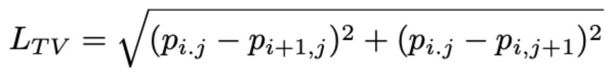
Equation 1. The loss function for total variation loss. Taken from [2]
- Testing was also performed on samples where portions of the face were obscured by surgical masks; the authors found that, in these cases, the amount of black used could be penalized to make the patches look more natural. They defined black penalty loss, Lblk, as the following for a given pixel p(i, j):
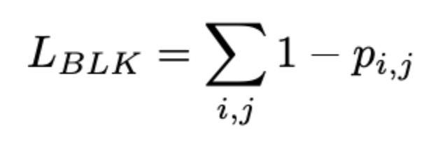
Equation 2. The loss function for black loss. Taken from [2]
Together, the total loss was defined using the function below, where α and β are scaling factors that control the contributions of total variance loss and black loss, respectively.
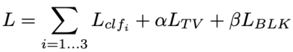
Equation 3. The loss function for the total loss, combining Lclf, Ltv and Lblk with their weighted factors. Taken from [2]
Both α and β were hyperparameters that were each individually optimized for. These three losses are evaluated together, summed, and back propagated to the patches for them to update. This training process continued for 2000 epochs per pair of patches.
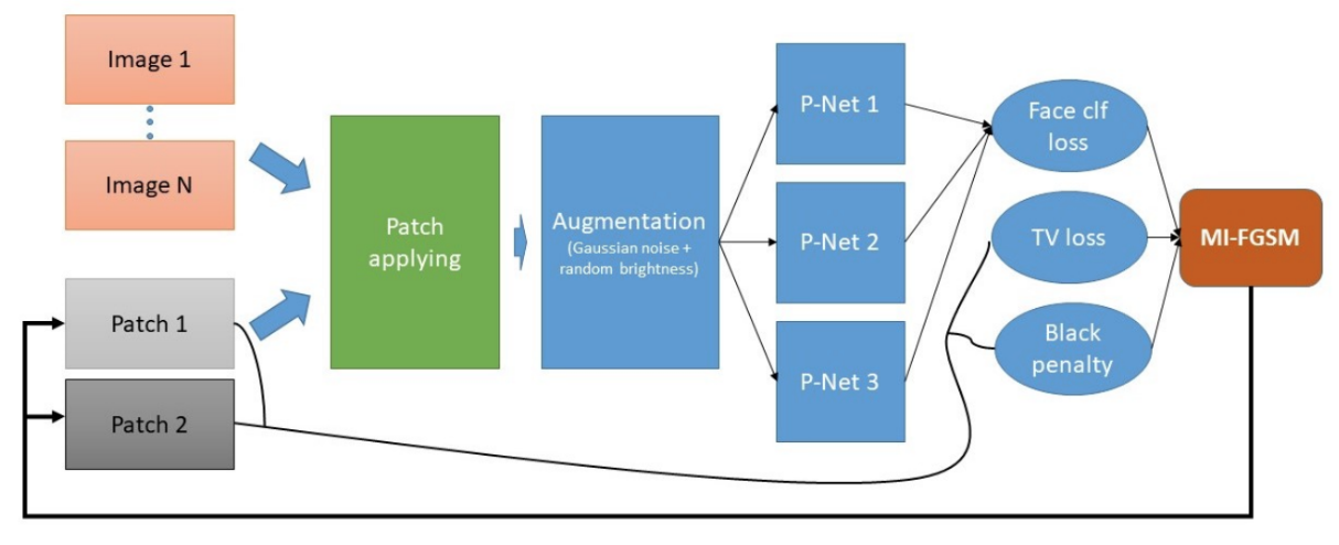
Fig. 4. The attack pipeline for MTCNN-Attack. A pair of patches is applied to N images and goes through data augmentation. The resulting images are fed through proposal networks to calculate classification loss, which is used alongside two other custom losses to update the patches through backpropagation. Taken from [2]
Another concern was the applicability of this methodology in real-time scenarios. In realistic cases, factors like lighting or angling differences could decrease the effectiveness of the patches. To account for this, Kaziakhmedov et al. used multiple images with different head positions and lighting for each sample, and marked each of the patch boundaries for each image. This allowed them to implement Expectation-over-Transformation (EoT) and projective transformations, which increase model effectiveness by ensuring that the patches are mapped correctly.
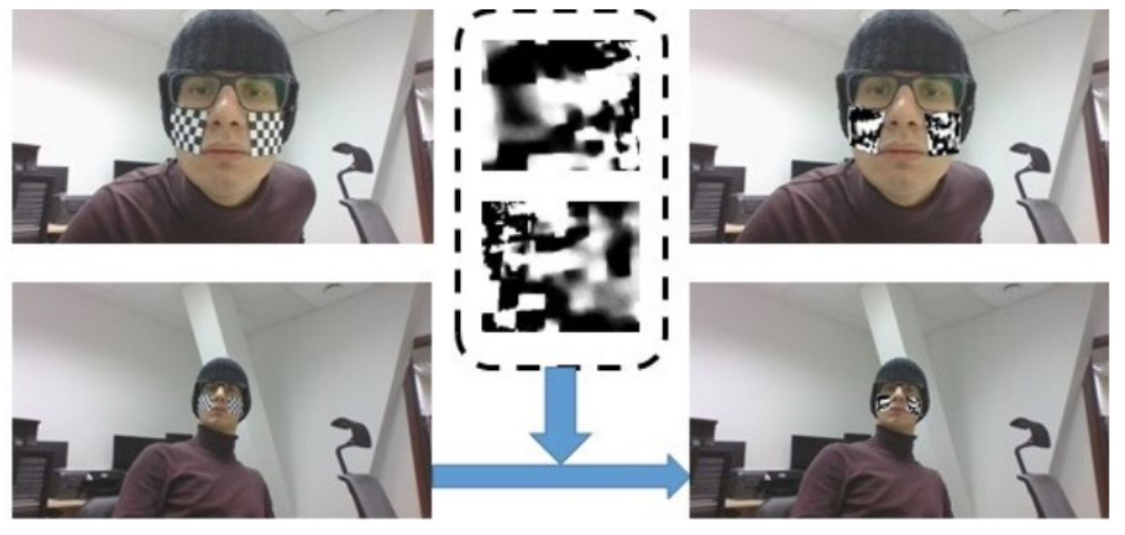
Fig. 5. An example of the sample input and the resultant patch mapping for the MTCNN-Attack model. Both EoT and projective mapping were used to ensure optimal patch placement. Taken from [2]
Results
Tests were performed to evaluate the probability of misdetection for both the bare-faced (cheeks) and masked datasets, and both unpatched and patched tests were considered. 2000 epochs were trained for the patches, and each result was averaged over a series of 1000 frames for each scale step factor. Scale step factors were valued at {0.709, 0.82, 0.9, and 0.95}. Over the range of scale steps, the probability of misdetection averaged slightly below 0.9 for the patched tests, and slightly below 0.2 for the unpatched for cheek; for masked, the model performed slightly worse, averaging slightly above 0.8 for patched and slightly above 0.2 for unpatched.
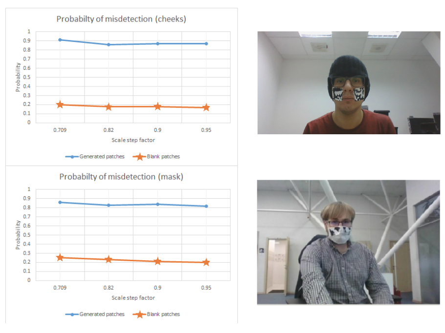
Fig. 6. The test results for both cheek and masked trials. Both tests show a strong misdetection performance for patched trials, especially when compared to unpatched trials. Taken from [2]
There are several issues that are worth consideration, however. Firstly, the completely unpatched database used to match patched and unpatched samples with people only contained images of the people in the sames (a “targeted” attack); this means that further investigation must be performed to evaluate whether or not the learned patches perform as well for the general human population, or whether transferability is an issue that must be addressed in the future. Secondly, there is an element of impracticality associated with this project, as one must be wearing the black-and-white checkered marks to denote where the patches should be located. Generally, this may be deemed unsuitable for everyday use. But overall, the results show a considerable improvement with the learned patches as opposed to unpatched, suggesting that the model conceivably could be used to prevent facial identification in the future.
Unlearnable Examples
Introduction
Unlearnable Examples is an AFR technique designed to render training data ineffective for Deep Neural Networks (DNNs). The primary objective is to ensure that DNNs trained on these modified examples perform no better than random guessing when evaluated on standard test datasets, while maintaining the visual quality of the data. For instance, an unlearnable selfie should remain visually appealing and suitable for use as a social profile picture, achieved by adding imperceptible noise that does not introduce noticeable defects.
DNNs are susceptible to adversarial, or error-maximizing, noise—small disturbances designed to increase a model’s error during testing However, applying this type of noise in a sample-wise manner during training does not effectively prevent DNNs from learning. To address this limitation, error-minimizing noise deceives the model into perceiving that there is no valuable information to learn from the training examples. This results in unlearnable examples that hinder the DNN’s ability to generalize, making its performance comparable to random guessing on standard test data.
Objectives
Suppose the clean training dataset consists of n clean examples, \(\mathbf{x} \in \mathbf{X}\) inputs, \(y \in \mathbf{Y} = \{1, \dots, K\}\) labels, and K total classes.
We denote its unlearnable version by \(\mathbf{D}_u = \{(\mathbf{x}_i, y_i)\}_{i=1}^n\), where \(\mathbf{x} = \mathbf{x} + \delta\) is the unlearnable version of training example \(\mathbf{x} \in \mathbf{D}_c\) and \(\delta \in \Delta \subset \mathbb{R}^d\) is the noise that makes x unlearnable.
The noise \(\delta\) is bounded by \(\|\delta\|_p \leq \epsilon\), where p is the \(\ell_p\) norm, and is set to be small such that it does not affect the normal utility of the example.
The DNN model will be trained on \(\mathbf{D}_c\) to learn the mapping from the input space to the label space: \(f : \mathbf{X} \rightarrow \mathbf{Y}\). The goal is to trick the model into learning a strong correlation between the noise and the labels: \(f : \Delta \rightarrow \mathbf{Y}, \Delta = \mathbf{X}\), when trained on \(\mathbf{D}_u\), the unlearnable version:
\[\arg\min_{\theta} \mathbb{E}_{(\mathbf{x}, y) \sim \mathbf{D}_u} \left[ L(f(\mathbf{x}), y) \right]\]where L is the classification loss such as the commonly used cross-entropy loss.
The noise forms are as follows: sample-wise noise, \(\mathbf{x}_i = \mathbf{x}_i + \delta_i\), \(\delta_i \in \Delta_s = \{\delta_1, \dots, \delta_n\}\), while for class-wise noise, \(\mathbf{x}_i = \mathbf{x}_i + \delta_{y_i}\), \(\delta_{y_i} \in \Delta_c = \{\delta_1, \dots, \delta_K\}\). Sample-wise noise requires generating unique noise for each individual example, which can limit its practicality. In contrast, class-wise noise applies the same noise to all examples within a specific class, making it more efficient and flexible for real-world applications. However, as we will observe, class-wise noise is more susceptible to detection and exposure.
Generating Error Minimizing Noise
Ideally, the noise should be generated on an additional dataset that is different from \(\mathbf{D}_c\). This will involve a class-matching process to find the most appropriate class from the additional dataset for each class to protect in \(\mathbf{D}_c\).
To generate the error-minimizing noise \(\delta\) for training input x, the following bi-level optimization problem is solved:
\[\arg\min_{\theta} \mathbb{E}_{(\mathbf{x}, y) \sim \mathbf{D}_c} \left[ \min_{\delta} L(f(\mathbf{x} + \delta), y) \right] \quad \text{s.t.} \quad \|\delta\|_p \leq \epsilon\]where f denotes the source model used for noise generation.
Note that this is a min-min optimization problem: the inner minimization is a constrained optimization problem that finds the \(\ell_p\)-norm bounded noise \(\delta\) that minimizes the model’s classification loss, while the outer minimization problem finds the parameters \(\theta\) that also minimize the model’s classification loss.
Noise Minimization Effectiveness
When class-wise noise is applied, both random and error-maximizing noise effectively prevent DNNs from learning useful information, particularly after the 15th epoch, highlighting the vulnerability of DNNs to such perturbations. However, these noise types can be partially circumvented by early stopping—for instance, halting training at epoch 15 can mitigate the impact of class-wise random noise.
Although error-maximizing noise is more challenging to overcome than random noise, as it only allows test accuracy to drop to around 50%, both methods remain only partially effective in making data unexploitable. In contrast, the proposed error-minimizing noise demonstrates greater flexibility and robustness, consistently reducing the model’s clean test accuracy to below 23% in both partially and fully unlearnable settings.
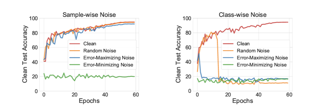
Fig 7. The unlearnable effectiveness of different types of noise: random, adversarial and error-minimizing noise on CIFAR-10 dataset. The lower the clean test accuracy the more effective of the noise. Taken from [3]
Class-wise noise introduces an explicit correlation with labels, causing the model to learn the noise instead of the actual content, which diminishes its ability to generalize to clean data. This type of noise also disrupts the independent and identically distributed (i.i.d.) assumption between training and test data, making it an effective data protection technique. However, class-wise noise can be partially bypassed through early stopping during training.
In contrast, sample-wise noise applies unique perturbations to each individual sample without any direct correlation to the labels. This approach ensures that only low-error samples are ignored by the model, while normal and high-error samples continue to aid in learning, making error-minimizing noise more effective in rendering data unlearnable. Consequently, sample-wise error-minimizing noise offers a more robust and versatile method for preventing DNNs from extracting useful information from the training data.
Experiment
Settings and Methodology
Huang et al. conducted a case study to demonstrate the application of error-minimizing noise on personal face images, addressing scenario where individuals seek to prevent their facial data from being exploited by FR or verification systems. This involves the defender applying error-minimizing noise to their own face images before sharing them on online social media platforms. These altered, or unlearnable, images are subsequently collected by FR systems to train DNNs. The primary objective is to ensure that DNNs trained on these unlearnable images perform poorly when attempting to recognize the defender’s clean face images captured elsewhere, thereby safeguarding the individual’s privacy.
The experiments are conducted under two distinct settings: partially unlearnable and fully unlearnable. In the partially unlearnable setting, a small subset of identities within the training dataset is made unlearnable. Specifically, 50 identities from the WebFace dataset are selected and augmented with error-minimizing noise using a smaller CelebA-100 subset.
This results in a training set where 10,525 identities remain clean, while 50 identities are protected. In the fully unlearnable setting, the entire WebFace training dataset is rendered unlearnable. Inception-ResNet models trained on these modified datasets evaluate the effectiveness of the noise against both face recognition and verification tasks.
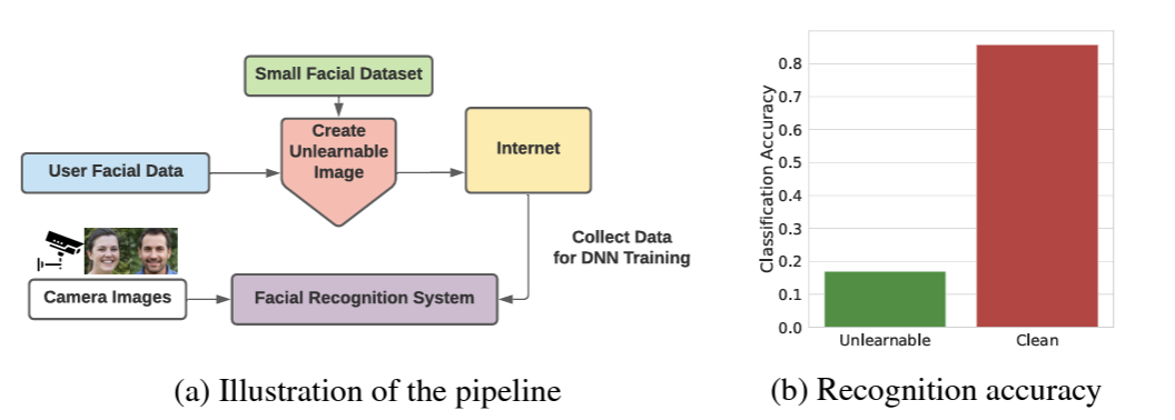
Fig 8. Preventing exploitation of face data using error-minimizing noise. Taken from [3]
Results
The study concludes that error-minimizing noise is a viable tool for protecting personal face images from unauthorized use in training FR systems. In the partially unlearnable setting, the recognition accuracy for the 50 protected identities dropped to 16%, compared to 86% for the remaining clean identities.
However, the partially unlearnable setting exhibits some limitations due to the presence of ample clean data, which allows the model to maintain relatively good verification performance, albeit with a reduced Area Under the Curve (AUC). In contrast, the fully unlearnable setting achieves a substantial reduction in model performance, with the AUC dropping from 0.9975 in the clean setting to 0.5321. This highlights the potential of error-minimizing noise for comprehensive data protection when applied across the entire dataset.
The findings suggest that error-minimizing noise can significantly enhance data privacy by making facial images unlearnable, thereby preventing DNNs from effectively utilizing such data for recognition or verification purposes. This advancement introduces a promising method for individuals to safeguard their personal information in an era of pervasive machine learning applications, ensuring that their facial data remains protected against unauthorized exploitation.
References
[1] Shan, Wenger, Zhang, Li, Zheng, Zhao. “Fawkes: Protecting Privacy against Unauthorized Deep Learning Models”. arXiv [cs.CV] 2020.
[2] Kaziakhmedov, Edgar, et al. “Real-world adversarial attack on MTCNN face detection system”. arXiv:1910.06261 [cs.CV]
[3] Huang, Hanxun, et al. “Unlearnable examples: Making personal data unexploitable.” arXiv preprint arXiv:2101.04898 (2021).
[4] Wenger, Emily, et al. “Sok: Anti-facial recognition technology.” 2023 IEEE Symposium on Security and Privacy (SP). IEEE, 2023.