Text-to-Image Generation
Text-to-image generation is a model that generates images from input text. Textual prompt is passed in as input, and the model outputs an image based on that prompt. We will be exploring the architecture and results of four text-to-image models: DALL-E, Imagen, Stable Diffusion, and GANs. We will also be running Stable Diffusion with WebUI and implementing subject-driven fine-tuning on diffusion models with Dreambooth’s method.
- DALL-E V1: Variational Autoencoder + Transformer
- Imagen: LLM + Diffusion Model
- Stable Diffusion
- GANs
- Running Stable Diffusion via WebUI
- Subject Driven Fine-tuning with Dreambooth
DALL-E V1: Variational Autoencoder + Transformer
The original DALL-E was based on the paper “Zero-Shot Text-to-Image Generation” by Aditya Ramesh et al in 2021. It was developed by OpenAI.
In this paper, the authors propose a 12-billion parameter autoregressive transformer trained on 250 million image-text pairs for text to image generation, claiming that not limiting models to small training sets could possibly produce better results for specific text prompts. It also achieves zero-shot image generation, meaning that the model produces high quality images for labels that it was not specifically trained on.
Method
The general idea for the model is to “train a transformer to autoregressively model the text and image tokens as a single stream of data” [1].
DALL-E’s training procedure consists of two stages:
Stage 1: Learning the Visual Codebook
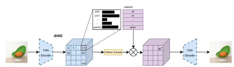
Figure 1. DALL-E’s dVAE autoencoder and decoder. [2]
- Train a discrete variational autoencoder (dVAE) to downsample the 256x256 RGB input image into a 32x32 grid, with each grid unit possibly having 1 of 8192 possible values from the 8192 codebook vectors trained during this stage.
- The codebook vectors contain discrete latent indices and its distribution via the input image
- A dVAE decoder is also trained on this step to be able to regenerate images from the discrete codes
- This step is also important for mapping the input data to discrete codebook vectors in latent space, where each code allows the model to capture categorical information about the image.
Stage 2: Learning the Prior
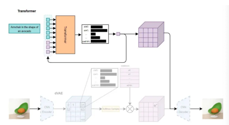
Figure 2. DALL-E’s transformer. [2]
- Concatenate up to 256 BPE-encoded (byte-pair encoded) text tokens with the 1024 image tokens and train an autoregressive transformer to model joint distribution over the tokens
- The transformer takes in text captions of training images and learns to produce the codebook vectors for one token, and then predicts the distribution for the next token until all 1024 tokens are produced.
- The dVAE decoder trained in stage 1 is used to generate the new image.
Loss Objective
The overall procedure maximizes the evidence lower bound (ELB) on the joint likelihood of the model distribution over images x, captions y, and tokens z for the encoded image.
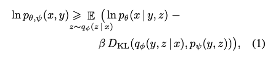
Figure 3. DALL-E’s loss objective. [1]
- q-phi is the distribution over image tokens given RGB input images
- p-theta is distribution over RGB images given image tokens
- p-psi is joint distribution over text and image tokens modeled by transformer
The goal of these stages is to reduce the amount of memory needed to train the model and to capture more low-frequency structure of the images rather than short-range dependencies between pixels that likelihood objectives tend to recognize.
Results
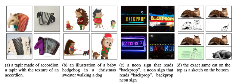
Figure 4. Text-to-image results from DALL-E v1. [1]
Here are some results from the initial DALL-E paper. This model architecture has been overtaken by recent models like diffusion models, which even DALL-E 2 and 3 are using. However, it is still interesting to study different text-to-image generation techniques.
Imagen: LLM + Diffusion Model
Imagen is a powerful text-to-image generation model developed by Google Brain which, at the time of its release, held the State of the Art performance on a variety of metrics, including the COCO FID benchmark. Key features of this innovative model are:
- LLM for text encoder
- Efficient UNet backbone
- Classifier-free guidance with dynamic thresholding
- Noise augmentation and conditioning in cascading diffusion models
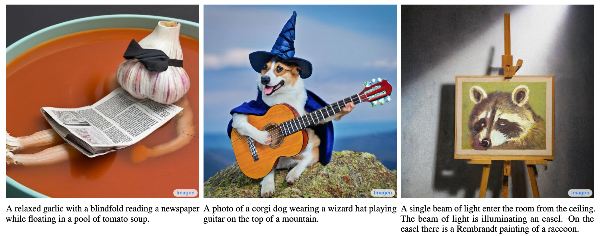
Fig 5. Examples of Imagen Generation [3]
Revisiting Diffusion Models
In Stable Diffusion, text conditioning is done via a separate transformer that encodes text prompts into the latent space of the diffusion model. These encoders are trained jointly with the diffusion backbone on pairs of images and their text captions. Thus, the text encoders are only exposed to a limited set of text data that is constrained to the space of image captioning and descriptors.
Although this method of jointly training a text encoder and diffusion model works well in practice, Imagen finds that using pre-trained large-language models has much better performance. In fact, Imagen uses the largest language model available at the time (T5-XXL) which is a general language model. The advantages of this approach are twofold, there is no need to train a dedicated encoder, and general encoders learn much better semantic information.
Not requiring a dedicated encoder makes the training process much easier, it is one less model that needs to be optimized. Using a separate and pre-trained model also allows training data to be directly encoded once, simplifying expensive computation that would have to be done for each training step. The Imagen authors state that text data is encoded one time, and that during training, the model can directly use (image, encoding) pairs rather than deriving encodings at every iteration from (image, text) pairs.
In addition, using pre-trained LLM allows the generative model to capitalize on important semantic representations already encoded and learned from vast datasets. Simply put, pre-trained models have a much better understanding of language since they are trained on much larger and richer data than dedicated diffusion text encoders.
The Imagen authors also report surprising results ‒ that the size of the language model has a direct correlation with better generative features. Scaling up the language model even has a much larger impact on generative capabilities than scaling the diffusion model itself.
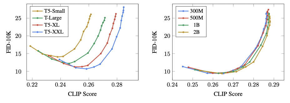
Fig 6. Imagen Experiments with Varying LLM and UNet size [3].
These charts, from the Imagen paper, show the model capabilities for varying sizes of LLM text encoders (on the left) and UNet diffusion models (on the right). Evidently, increasing the size of the text encoder has a much more drastic improvement on evaluation metrics than increasing the size of the diffusion backbone. A bigger text encoder equals a better generative model.
Imagen also adapts the diffusion backbone itself, introducing a new variant they call Efficient UNet. This version of the UNet model has considerably better memory efficiency, inference time, and convergence speed, being 2-3x faster than other UNets. Better sample quality and faster inference is essential for generative performance and training.
Further Optimizations
Imagen also introduces several other novel optimizations for the training process on top of revamping the diffusion backbone and text encoder. These optimizations include dynamic thresholding to enable aggressive classifier-free guidance as well as injecting noise augmentation and conditioning to boost upsampling quality.
Classifier-free guidance is a technique used to improve the quality of text conditional training in diffusion models. Its counterpart, classifier guidance, has the effect of improving sample quality while reducing diversity in conditional diffusion. However, classifier guidance involves pre-trained models that themselves need to be optimized. Classifier-free guidance is an alternative that avoids pre-trained models by jointly training a single diffusion model on conditional and unconditional objectives by randomly dropping the condition during training. The strength of classifier-free guidance is also controlled by a weight parameter.
Larger weights of classifier-free guidance improves text-image alignment but results in very saturated and unnatural images. Imagen addresses this issue with dynamic thresholding. In short, large weights on guidance pushes the values of the predicted image outside of the bounds of the training data (which are between -1, and 1). Runaway values lead to saturation. Dynamic thresholding constraints large values in the predicted image so that the resulting images are not overly saturated. The use of dynamic thresholding thus allows the use of aggressive guidance weights, which improve the model quality without leading to unnatural images.
In addition, the Imagen architecture also implements cascading diffusion models. The first DM generates a 64x64 image, then the second upsamples to 256x256, and the final upsamples to 1024x1024. This cascading method results in very high fidelity images. Imagen further builds on this capability by introducing noise conditioning and augmentations in the cascading steps.
Noise augmentation adds a random amount of noise to intermediate images between upsampling. Noise conditioning in the upsampling models means that the amount of noise added in the form of augmentations is provided as a further condition to the upsampling model.
These techniques, taken together, boost the quality produced by the final Imagen model.
Overview of Imagen Architecture
First, text prompts are passed to a frozen text encoder that results in embeddings. These embeddings are inputs into a text-to-image diffusion model that outputs a 64x64 image.
Then, the image is upsampled via two super-resolution models that create the final 1024x1024 image.
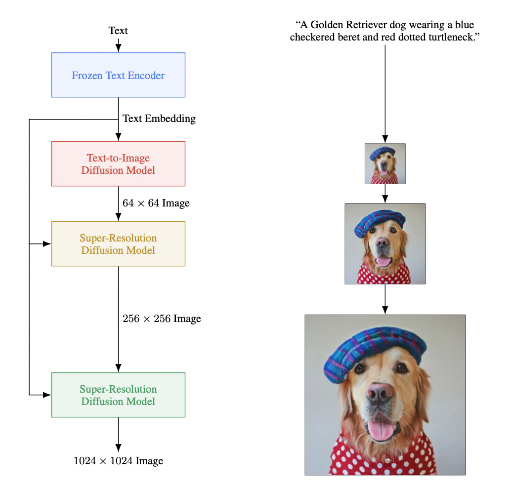
Fig 7. Imagen Architecture [3].
Stable Diffusion
As introduced above Diffusion Models are a class of likelihood-based models that use excessive amounts of capacity and resources for modeling finer details of data, thus have a high computational overhead. For example, training powerful Diffusion Models could take hundreds of GPU days. The solution that the paper, High-Resolution Image Synthesis with Latent Diffusion Models, presents is the Latent Diffusion Model, which addresses this limitation by training the autoencoder to provide a lower-dimensional representational space. The autoencoder only needs to be trained once and can be reused for multiple Diffusion Model training iterations.
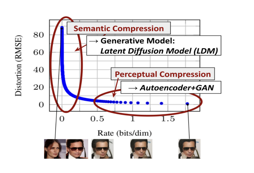
Figure 8. LDM removing finer details during semantic compression then generating the image. [4].
The Latent Diffusion Model process begins with an encoder ε that takes in an input image x in the RGB space with a shape of [H,W,3], and encodes x into a lower dimension representation z. The encoder extracts the most important features in z, which is referred to as the latent space and can be represented as z = ε(x). The latent space is then downsampled by factor f, a hyperparameter, resulting in latent representation z being smaller than input image x. The latent space is reconstructed using a decoder which can be represented as D(z) = x̂, where x̂ is the reconstructed image and an approximation of the original image x.
The advantage of Latent Diffusion models is that it preserves the 2D spatial relationships and structure, unlike previous work where the input was flattened into most commonly a 1D vector thus losing critical structural information. Thus Latent Diffusion Models learns representation in lower-dimensional space in order to capture meaningful structure and through denoising removes fine-grained details which decreases the overall computational overhead, without affecting the model’s overall performance when generating high-quality images.
Loss Objective
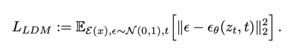
Figure 9. Latent Diffusion Model’s loss objective. [4].
The loss function of the Latent Diffusion Model aims to minimize the difference between the actual noise and predicted noise from the latent space, z, in order to train the neural network to learn to predict noise introduced during the forward diffusion process. Additionally, Kullback-Leibler regularization term added to the loss function penalizes deviation from the normal standard distribution in order to reduce variance/overfitting.
GANs
Generative Adversarial Networks (GANs) is a deep generative model first introduced in the paper “Generative Adversarial Nets”, proposed by Ian Goodfellow and his colleagues. The idea behind GANs is to simultaneously train two neural networks–a generator \(G\) and a discriminator \(D\)–to compete against each other. \(G\) creates fake data to deceive \(D\) as real data while \(D\) attempts to accurately distinguish the generated data from real data. The significance of this adversarial nets framework is that both \(D\) and \(G\) can be trained with backpropagation and that Markov chains or inference networks are not required. GANs have set the foundation of deep generative models as they output high-quality results based on complicated data distributions. Today, they are applied in a wide variety of fields including video prediction, super-resolution, and text-to-image generation. However, there are challenges such as unstable training and difficulty in tuning hyperparameters.
Overview of GANs
The general setup for adversarial training of GANs is as follows: [5]
- Generator (\(G\)): The generator learns to map random noise to data samples. The goal is to create data that is indistinguishable from the real dataset.
- Discriminator (\(D\)): The discriminator performs as a binary classifier that assumes 0 for fake and 1 for real data.
- Loss Functions: GANs use two loss functions:
- The objective of \(D\)’s loss function is to maximize its accuracy in classifying real and fake data.
- The objective of \(G\)’s loss function is to minimize D’s ability to correctly label generated data.
Over the data \(\boldsymbol{x}\), the generator synthesizes its distribution \(p_{\boldsymbol{z}}(\boldsymbol{z})\) and maps it to data space \(G(\boldsymbol{z};\theta_{g})\) to obtain the distribution \(p_{g}\) in the end. Here, \(G(\boldsymbol{z};\theta_{g})\) is a differentiable function that is a representation of a multilayer perceptron. There is another multilayer perceptron \(D(\boldsymbol{x};\theta_{d})\) that outputs a scalar value probability of if \(\boldsymbol{x}\) is derived from data rather than \(p_{g}\). The goal of \(D(\boldsymbol{x})\) is to maximize the probability of correctly discriminating training examples and samples by minimizing \(\log(1 - D(G(\boldsymbol{z})))\). That is, \(D\) and \(G\) compete against each other with the value function \(V(G, D)\). The following is the mathematical representation of the objective function:

Fig 10. Value Function of GANs [5].
Note that in reality, the above equation is not good enough for \(G\) to learn effectively, especially in the early stage of learning. When \(G\) is not optimized yet, \(D\) can confidently reject the generator’s output as fake. As a result, \(\log(1 - D(G(\boldsymbol{z})))\) approaches 0, and the learning becomes harder. In this step, \(G\) is trained to maximize \(\log(D(G(\boldsymbol{z})))\) instead.
Below is the visual interpretation of the training progress of \(G\) and \(D\). The black dotted line represents \(p_{x}\) or the true data distribution. The green solid line represents \(p_{g}\), the generated data distribution, which is the distribution of samples created by \(G\). The blue dashed line is \(D\). In the final step of the training, Both \(G\) and \(D\) reach the equilibrium where \(p_{g} = p_{\text{data}}\) and \(D(\boldsymbol{x}) = \frac{1}{2}\).
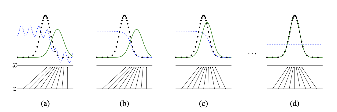
Fig 11. GANs: Training Process of Generator and Discriminator [5].
Here is a visualization of GANs outputs. Yellow boxes are the nearest training examples generated by GANs trained with different datasets: a. MNIST, b. TFD, c. and d. CIFAR-10.
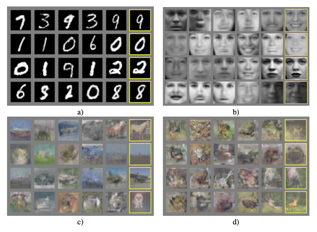
Fig 12. GANs: Generated Sample Images Trained on Different Datasets [5].
Future Improvements
GANs have a significant advantage as unsupervised learning that doesn’t require labeled data. They are now developed into diverse variations: StyleGAN can produce high-quality image synthesis and Pix2Pix or CycleGAN can be utilized in versatile applications. On the other hand, they still have room for improvement to resolve some problems such as the generator’s mode collapse, unstable training, and imperfect evaluation metrics.
Comparison with Stable Diffusion
Stable Diffusion can be an alternative approach to generate images. It has some advantages over GANs:
- Stable Diffusion or Latent Diffusion Models iteratively refine noisy input to produce coherent outputs, and the training procedure is more robust.
- It has more diversity in generated samples while GANs can suffer from mode collapse. However, GANs are more efficient in terms of computation compared to Stable Diffusion and better at creating highly realistic samples that resemble real life. Both GANs and Stable Diffusion are remarkable generative models, so it is crucial to weigh costs and benefits of both models to choose a more appropriate one for an intended purpose.
Running Stable Diffusion via WebUI
Our group decided to use AUTOMATIC1111’s stable diffusion web UI to run pre-existing stable diffusion models.
Introduction to Stable Diffusion Web UI
Stable Diffusion Web UI is a web interface for Stable Diffusion, which provides traditional image to image and text to image capabilities. It also provides features like prompt matrices, where you can provide multiple prompts and a matrix of multiple images will be produced based on the combination of those prompts.
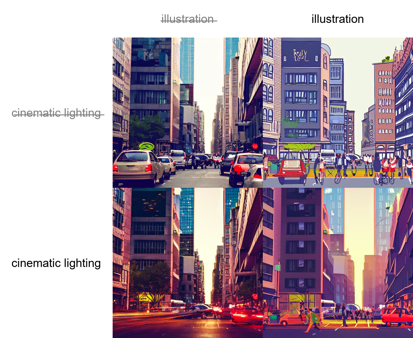
Figure 13. Prompt matrix. Several images all with the same seed are produced based on the combination of the prompts “a busy city street in a modern city|illustration|cinematic lighting,” where | indicates the separation of prompts. [6].
In addition, it provides an Attention feature where using () in the text prompt increases the model’s attention on those enclosed words, and using [] decreases it. Adding more () or [] around the same enclosed words increases the magnitude of the effect.
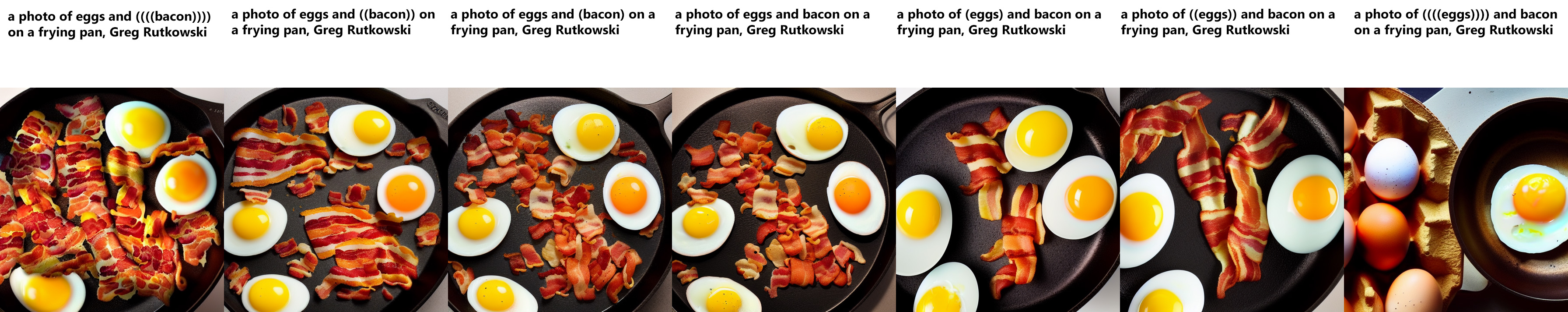
Figure 14. Attention. Web UI provides features to increase and decrease attention on specific words in text prompt. [6].
Guide on Running Web UI
This is a small guide on how to run stable diffusion models using Stable Diffusion web UI on Mac. It is based on this tutorial.
Step 1: Install Homebrew and add brew to your path
/bin/bash -c "$(curl -fsSL https://raw.githubusercontent.com/Homebrew/install/HEAD/install.sh)"
Add brew to your path
echo 'eval $(/opt/homebrew/bin/brew shellenv)' >> /Users/$USER/.zprofile
eval $(/opt/homebrew/bin/brew shellenv)
Step 2: Install required packages
brew install python@3.10 git wget
Step 3: Clone AUTOMATIC1111 webui repo
git clone https://github.com/AUTOMATIC1111/stable-diffusion-webui [location on your disk]
A stable-diffusion-webui folder should’ve been created wherever you specified the git clone destination to be.
Step 4: Run AUTOMATIC1111 webui
cd [destination dir]/stable-diffusion-webui
./webui.sh
After a while a new browser page hosted at http://127.0.0.1:7860/ should open.
Astronaut Cat: Playing Around with Stable Diffusion Web UI’s Text to Image Functionalities
Our team decided to explore web UI’s text to image functionalities using the prompt “astronaut cat” (because why not :)).
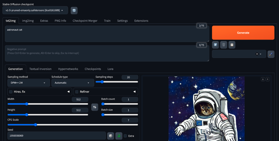
Figure 15. First look at web UI’s txt2img functionality with the prompt “astronaut cat.”
The first thing to note from Figure 15 is that web UI allows us to change the Stable Diffusion checkpoint that we wish to use. By default following the guide above, the checkpoint is v1-5-pruned-emaonly.safetensors.
Next, the various tabs right below the Stable Diffusion checkpoint field show the various features that web UI provides, including img2img, embedding and hypernetwork training, and a place to allow users to upload their own PNGs. We will be focusing on the txt2img tab.
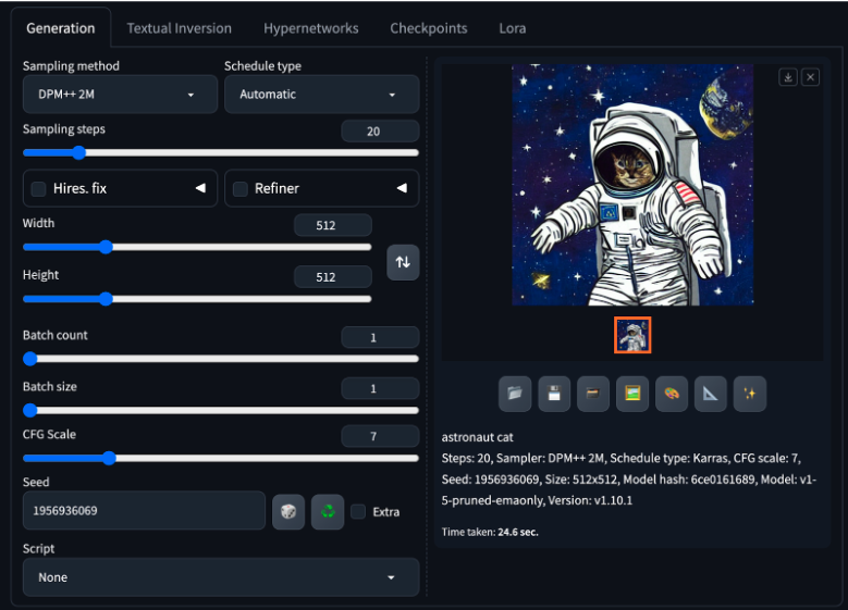
Figure 16. Web UI allows the user to change the sampling method, schedule type, sampling steps, batch size, CGF scale, seed, and much more for image generation, all in a nice interface.
For text to image, web UI provides many easy-to-use interfaces to change parameters for image generation. For example, you can specify the sampling method or the schedule type that you want. You can also specify the number of sampling steps, image size, batch count and size, CFG scale, and seed. You can also upload custom scripts that can add even more functionality to web UI such as generating color palettes by text prompt or specifying inpainting mask through text rather than manually drawing it out.
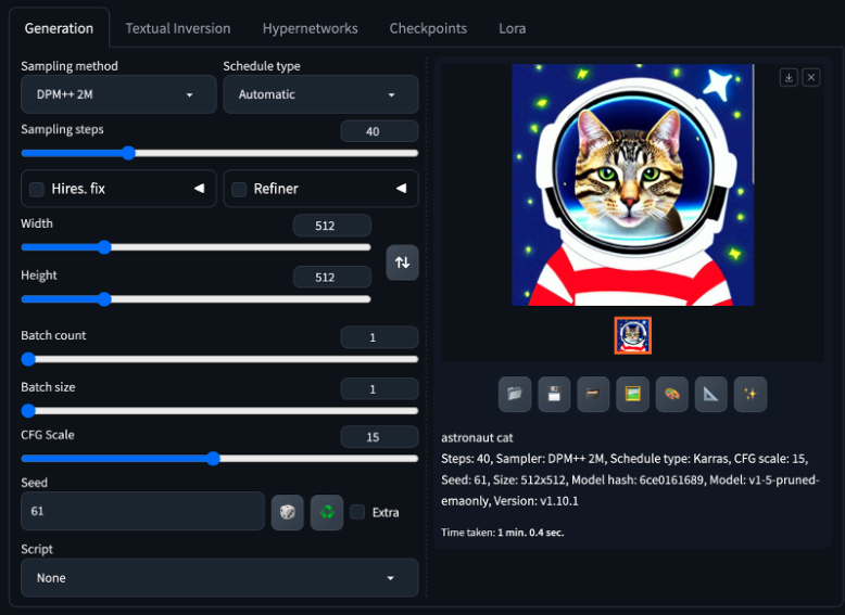
Figure 17. Astronaut cat with some modified parameters.
Playing around with some parameters (which is easy with the slider interface), we tested increasing the sampling steps by a little and increasing the CFG scale to 15, as well as setting the seed to 61. Figure 17 shows the results, which shows the cat in a forward-facing position and more realistic features (although the suit remains animated).
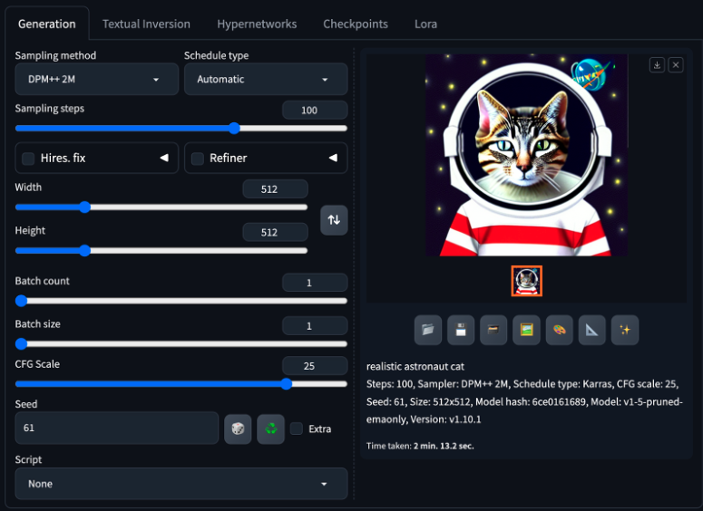
Figure 18. Making the image more realistic by increasing sampling steps and CFG scale, as well as changing the prompt to “realistic astronaut cat”.
Changing the prompt to “realistic astronaut cat”, increasing the sampling steps, and increasing the CFG scale even more produces an even more realistic cat, and this time the suit has some 3-dimensional shading and the background is more detailed.
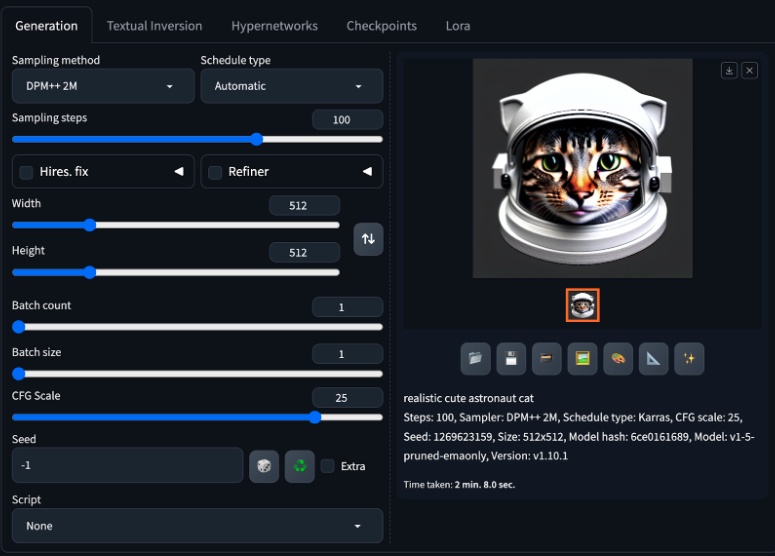
Figure 19. Attempt to produce a cute astronaut cat.
Finally, in the desire to produce a cute astronaut cat, we changed the prompt to “realistic cute astronaut cat” and set the seed to random, which produced this rather cute cat with an astronaut helmet with cat ears!
Subject Driven Fine-tuning with Dreambooth
Leveraging generative data for downstream tasks typically requires some degree of subject driven fine-tuning. In these cases, the concern is how to guide generative outputs to match the appearance of subject inputs. Dreambooth is a method for such tuning.
For example, lets say a user wants to generate images of their pet cat in various environments and poses. Passing a text prompt describing their cat leads to outputs that may look unnatural and unrepresentative of the beloved household feline in question.
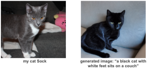
Figure 20. Attempt to generate image of my cat, Sock, with out-of-box diffusion model
However, the Dreambooth method allows such targeted subject generation. The key is that instead of explicitly describing the subject characteristics, Dreambooth fine-tunes a model to directly attach those characteristics to a specific text keyword. The model learns to associate a given subject with this keyword and when prompted with the same keyword, is able to generate very realistic images of the input subject.
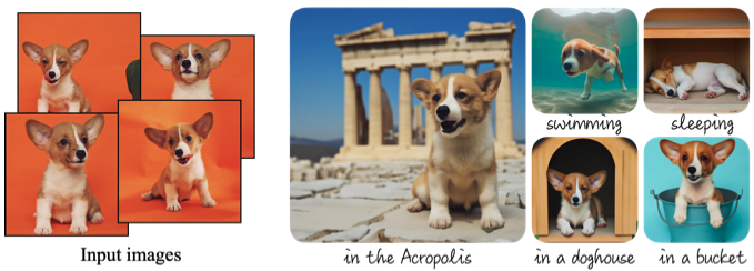 Figure 21. Examples of Dreambooth Subject-Driven Fine Tuning [7].
In fact, the keywords themselves are already present in the model, although it is a requirement that these rare tokens do not already have semantic meanings attached to them. A notable example is the phrase “sks”. This phrase, which is already a part of the text encoders vocabulary, has no semantic meaning associated with it. By tuning a model on subject images with the text embedding “a sks [class]”, the model is able to tie the subject information with the keyword. Subsequent generations using the token “sks” will reproduce the subject in the output.
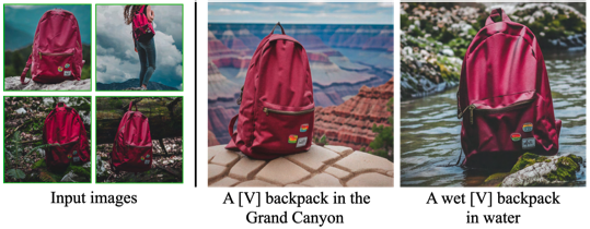 Figure 22. Examples of Dreambooth Generation with Rare Tokens [7].
Implementing Dreambooth to Generate Pictures of my Cat
To explore the capabilities of subject-driven generation, I used my cat Sock as an example. The code that follows is adapted from Huggingface’s Dreambooth training script. You can see my annotated notebook here.
Tuning a model to generate pictures of Sock via Dreambooth is deceptively simple. First, a rare token needs to be selected, in this case the ubiquitous “sks”. Then, from only three subject images, all attached with the same prompt, “a sks cat…”, the model will become personalized to the subject.
First, a dataset is needed to store the subject images and pair them with the input prompts.
Class DreamBoothDataset(Dataset):
  """
  A dataset to preprocess instances for fine-tuning model. Pre-processes the images and tokenizes prompts.
  """
  def __init__(self,
               instance_data_root,
               instance_prompt,
               tokenizer,
               size=512,
               center_crop=False):
    # saving args
    self.size = size
    self.center_crop = center_crop
    self.tokenizer = tokenizer

    # saving root (instance root is path to folder containing image)
    self.instance_data_root = Path(instance_data_root)
    # check if root exists
    if not self.instance_data_root.exists():
      raise ValueError(f"Instance {self.instance_data_root} root doesn't exist.")

    # initializing list with paths of all images in instance root
    self.instance_images_path = list(Path(instance_data_root).iterdir())
    # length
    self.num_instance_images = len(self.instance_images_path)
    self._length = self.num_instance_images

    # saving prompt (same for all images in instance)
    self.instance_prompt = instance_prompt

    # initializing transforms
    self.image_transforms = transforms.Compose([
        transforms.Resize(size, interpolation=transforms.InterpolationMode.BILINEAR),
        transforms.CenterCrop(size) if center_crop else transforms.RandomCrop(size),
        transforms.ToTensor(),
        transforms.Normalize([0.5], [0.5])
    ])

    # other functions omitted, see attached notebook or Hugginface script
Then, load the diffusion models components: tokenizer and text encoder for text prompts, noise scheduler, text encoder, VAE, and diffusion UNet backbone. Some helper functions and arguments ommitted, please see notebook or Huggingface script
# load tokenizer
tokenizer = AutoTokenizer.from_pretrained(
    args.pretrained_model_name_or_path,   # args is a structure of training arguements
    subfolder = "tokenizer",
    use_fast = False
)
# import text encoder class
text_encoder_cls = import_model_class_from_model_name_or_path(args.pretrained_model_name_or_path)

# load scheduler and models
noise_scheduler = DDPMScheduler.from_pretrained(args.pretrained_model_name_or_path, subfolder="scheduler")
text_encoder = text_encoder_cls.from_pretrained(
    args.pretrained_model_name_or_path, subfolder="text_encoder"
)
vae = AutoencoderKL.from_pretrained(args.pretrained_model_name_or_path, subfolder="vae")
unet = UNet2DConditionModel.from_pretrained(
    args.pretrained_model_name_or_path, subfolder="unet"
)
Make sure the VAE and text encoders are frozen (only training diffusion backbone).
# will not be training text or image encoders
vae.requires_grad_(False)
text_encoder.requires_grad_(False)
Initilize the optimizer, dataset, and learning rate scheduler.
# create optimizer
optimizer = optimizer_class(
    unet.parameters(),
    lr = args.learning_rate,
    betas = (args.adam_beta1, args.adam_beta2),
    weight_decay = args.adam_weight_decay,
    eps = args.adam_epsilon
)

# load dataset and dataloader
train_dataset = DreamBoothDataset(
    instance_data_root = args.instance_data_dir,
    instance_prompt = args.instance_prompt,
    tokenizer = tokenizer,
    size = args.resolution,
    center_crop = args.center_crop
)

train_dataloader = torch.utils.data.DataLoader(
    train_dataset,
    batch_size = args.train_batch_size,
    shuffle = True,
    collate_fn = lambda examples: collate_fn(examples),
    num_workers = 2
)

# setting up lr scheduler
lr_scheduler = get_scheduler(
    args.lr_scheduler,
    optimizer = optimizer,
    num_warmup_steps = args.lr_warmup_steps * args.gradient_accumulation_steps,
    num_training_steps = args.max_train_steps * args.gradient_accumulation_steps,
    num_cycles = args.lr_num_cycles,
    power = args.lr_power
)
And train!
After only 200 iterations on 3 subject image inputs, the model can generate very realistic images.
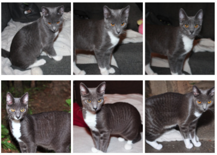
Figure 23. Personalized Dreambooth Outputs. Top row is original image, bottom row is generated outputs
Applications of Subject-Driven Generation: Generative Data Augmentation
The subject of generative data augmentation has already been used in a variety of applications where training data is extremely scarce. In these situations, generated data is used to artificially expand the training dataset and enable model training.
A key concern when training models on generated data is ensuring that the artificial data points are relevant, that they accurately represent their real counterparts.
To tackle this key issue, precise subject-driven generative models are used to create realistic and meaningful training data.
Figure 24. Examples of GDA from DATUM Paper [8].
References
[1] Ramesh, Aditya, et al. “Zero-Shot Text-to-Image Generation.” Proceedings of the 38th International Conference on Machine Learning. 2021.
[2] Abideen, Zain ul. “How OpenAI’s DALL-E works?” Medium. 2023.
[3] Saharia, Chitwan, et al. “Photorealistic text-to-image diffusion models with deep language understanding.” arXiv preprint arXiv:2205.11487 2022.
[4] Rombach, Robin, et al. “High-Resolution Image Synthesis with Latent Diffusion Models.” arXiv preprint arXiv:2112.10752. 2022.
[5] Goodfellow, Ian J., et al., “Generative Adversarial Networks.” arXiv. doi: 10.48550/ARXIV.1406.2661. 2014.
[6] AUTOMATIC1111. “stable-diffusion-webui-feature-showcase”. Github.
[7] Ruiz, Nataniel, et al. “DreamBooth: Fine Tuning Text-to-Image Diffusion Models for Subject-Driven Generation.” arXiv preprint arXiv:2208.12242. 2023.
[8] Benigmim, Yasser, et al. “One-shot Unsupervised Domain Adaptation with Personalized Diffusion Models.” arXiv preprint arXiv:2303.18080. 2023.