Image Super Resolution
This post compares and contrasts three methods of performing image super resolution: Enhanced Deep Residual Networks (EDSR), Residual Channel Attention Networks (RCAN), and Residual Dense Networks (RDN). In addition, we experiment with finetuning one of these networks on the MiniPlaces dataset.
- Introduction
- Enhanced Deep Residual Networks (EDSR)
- Residual Channel Attention Networks (RCAN)
- Residual Dense Networks (RDN)
- Implementing our Own Experiment
- Overall Discussion and Future Work
- Conclusion and Takeaways
- References
Introduction
Image Super-Resolution (SR) is a critical area in computer vision that aims to reconstruct high-resolution (HR) images from low-resolution (LR) inputs by restoring fine details and high-frequency features. This process is essential in applications where visual precision is crucial, including medical imaging, satellite surveillance, video streaming, and security systems. The core challenge of SR lies in reconstructing visually accurate details while mitigating common issues like blurring, noise, and compression artifacts. Traditional interpolation-based methods, such as bicubic upscaling, often fail to recover fine textures and structural details due to their limited feature-extraction capabilities. With the advancement of deep learning, convolutional neural networks (CNNs) have emerged as the state-of-the-art solution for SR. Modern SR architectures leverage innovative designs like residual learning, attention mechanisms, and dense feature fusion to significantly improve reconstruction accuracy. Among these, Enhanced Deep Residual Networks (EDSR), Residual Channel Attention Networks (RCAN), and Residual Dense Networks (RDN) have set new performance benchmarks across major SR datasets like DIV2K, Set5, and Urban100. This post investigates these three architectures, providing an in-depth analysis of their design principles, unique features, and performance metrics. We aim to highlight how each model addresses specific SR challenges through architectural innovations.
Enhanced Deep Residual Networks (EDSR)
The EDSR architecture effectively addresses the limitations of previous deep SR networks by removing batch normalization and employing residual scaling. These architectural refinements allow the model to become much deeper and wider, capturing more intricate image details. As a result, EDSR consistently outperforms prior methods, achieving higher PSNR/SSIM scores and producing more visually convincing high-resolution images. Moreover, the introduction of MDSR demonstrates the flexibility of the approach, enabling a single network to handle multiple upscaling factors efficiently. Although this comes at the cost of greater computational demands, the performance gains and versatility make EDSR and MDSR valuable solutions for tasks that require superior image quality, such as medical imaging, satellite imagery analysis, and professional photo enhancement.
Key Concepts
- Removal of Unnecessary Modules: By eliminating batch normalization layers, EDSR frees the network from normalization constraints. This enables deeper and wider architectures without introducing training instability.
- Residual Scaling and Increased Capacity: EDSR uses a residual scaling factor (e.g., 0.1) after each residual block. This allows the network to safely handle a large number of filters and many residual blocks, thus improving representational power and output quality.
Architecture
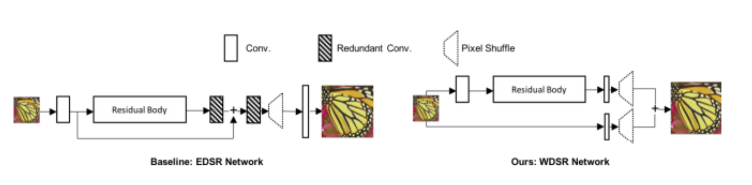
Figure 1. The EDSR network structure. [1].
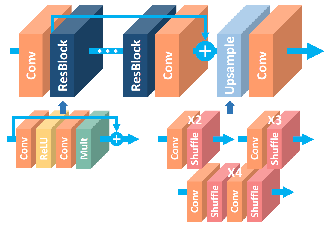
Figure 2. The architecture of the proposed single-scale SR network (EDSR). [1].
- Shallow Feature Extraction: The low-resolution (LR) input image first passes through an initial convolutional layer to extract basic feature maps, serving as the input to subsequent residual blocks.
- Residual Blocks (No BN): Each residual block consists of two convolutional layers separated by a ReLU activation. Crucially, no batch normalization layers are used, allowing the network to learn richer features. A residual scaling factor is applied at the end of each block, stabilizing training while enabling deep architectures.
- Global Skip Connection: Similar to other residual networks, a global skip connection is employed. It provides a direct pathway from the shallow features to the final layers, ensuring that low-frequency information is preserved while the stacked residual blocks focus on adding high-frequency details.
- Upscale Module: After extracting and refining features, the network uses an upsampling module, often a pixel shuffle (sub-pixel convolution) layer, to increase the spatial resolution. This step maps the learned high-dimensional features back to the high-resolution space.
- Single-Scale and Multi-Scale (MDSR) Variants:
- Single-Scale EDSR: Optimized for a particular upscaling factor, it achieves state-of-the-art results by tailoring the network depth and width to a single scale.
- MDSR: Extends EDSR to handle multiple scales (e.g., ×2, ×3, ×4) in one model by adding scale-specific pre-processing and upsampling layers, while sharing a large body of residual blocks across all scales. This reduces parameter counts and training complexity compared to having separate models for each scale.
Key Results
- PSNR (Peak Signal-to-Noise Ratio): EDSR achieves significant improvements in PSNR compared to earlier methods. For example, on the Set5 dataset, EDSR surpasses previous methods like VDSR and SRResNet, indicating sharper and more detailed reconstructions.
- SSIM (Structural Similarity Index): EDSR maintains high SSIM values, reflecting improved structural fidelity and texture preservation in the reconstructed high-resolution images.
- Performance on Benchmarks: EDSR (and MDSR) sets new state-of-the-art scores on multiple benchmark datasets such as Set5, Set14, B100, Urban100, and DIV2K. Its superior performance was confirmed by winning top places in the NTIRE2017 Super-Resolution Challenge.
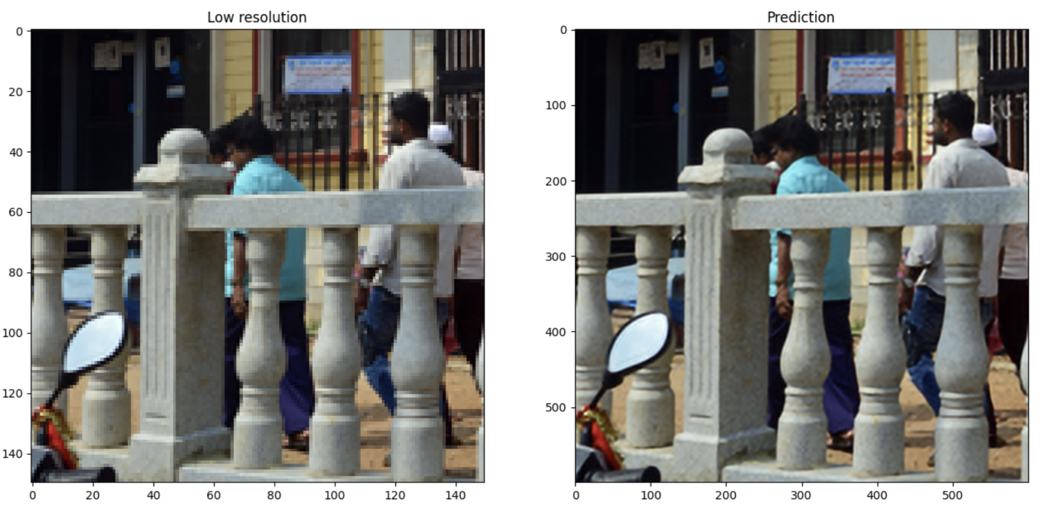
Figure 3. A prediction made by the EDSR network. [1].
Residual Channel Attention Networks (RCAN)
The RCAN architecture effectively deals with the challenge of training extremely deep neural networks by leveraging the RIR structure. This design allows the network to bypass low-frequency information and focus on high-frequency details critical for SR tasks. The inclusion of CA enhances this ability by dynamically adjusting the importance of features, ensuring that essential details are amplified. Experimental results demonstrate that RCAN achieves superior performance on standard benchmarks like Set5, Urban100, and Manga109. Its ability to maintain high PSNR and SSIM values while preserving fine details makes it highly effective in applications requiring precise image reconstruction.
Key Concepts
RCAN addresses challenges in SR by introducing two key concepts:
- Residual in Residual (RIR) Structure: This structure enables deep learning by stacking multiple residual groups (RGs), each containing several residual channel attention blocks (RCABs). Long and short skip connections facilitate information flow and bypass low-frequency components.
- Channel Attention (CA) Mechanism: This mechanism adaptively resizes channel-wise features by modeling interdependencies, allowing the network to prioritize high-frequency details such as edges and textures.
Architecture
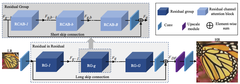
Figure 4. The RCAN architecture. [2]. RCAN employs a hierarchical design with the following components:
- Shallow Feature Extraction: The LR input image first passes through a convolutional layer to extract basic features.
- Residual Groups (RGs): Multiple RGs, each consisting of stacked Residual Channel Attention Blocks (RCABs), are the core of the network. Each RG has:
- RCABs: These blocks incorporate channel attention to amplify significant features while suppressing redundant information. Each RCAB contains a short skip connection, allowing the bypass of low-frequency data within the group.
- Short Skip Connections: Enable the network to stabilize and accelerate training by directly passing certain features to subsequent layers.
- Long Skip Connections: Connect the output of each RG directly to the final output of the RIR module, ensuring effective propagation of global information across the network.
- Upscale Module: After feature extraction, the network employs an upscale module to increase spatial resolution using techniques like transposed convolutions.
- Reconstruction Layer: The final convolutional layer reconstructs the HR output from the upscaled feature map.
Key Results
| Method | Scale | Set5 PSNR | Set5 SSIM | Set14 PSNR | Set14 SSIM | B100 PSNR | B100 SSIM | Urban100 PSNR | Urban100 SSIM | Manga109 PSNR | Manga109 SSIM |
|---|---|---|---|---|---|---|---|---|---|---|---|
| Bicubic | x3 | 28.78 | 0.8308 | 26.38 | 0.7271 | 26.33 | 0.6918 | 23.52 | 0.6862 | 25.46 | 0.8149 |
| SPMSR | x3 | 32.21 | 0.9001 | 28.89 | 0.8105 | 28.13 | 0.7740 | 25.84 | 0.7856 | 29.64 | 0.9003 |
| SRCNN | x3 | 32.05 | 0.8948 | 28.80 | 0.8074 | 28.13 | 0.7736 | 25.70 | 0.7770 | 29.47 | 0.8924 |
| FSRCNN | x3 | 26.23 | 0.8124 | 24.44 | 0.7106 | 24.86 | 0.6832 | 22.04 | 0.6745 | 22.39 | 0.7927 |
| VDSR | x3 | 33.25 | 0.9150 | 29.39 | 0.8310 | 28.53 | 0.7893 | 26.66 | 0.8136 | 31.35 | 0.9234 |
| IRCNN | x3 | 33.38 | 0.9182 | 29.63 | 0.8248 | 28.64 | 0.7942 | 26.77 | 0.8154 | 31.63 | 0.9245 |
| SRMDNF | x3 | 34.01 | 0.9242 | 30.11 | 0.8364 | 28.98 | 0.8009 | 27.50 | 0.8370 | 32.07 | 0.9391 |
| RDN | x3 | 34.58 | 0.9280 | 30.52 | 0.8462 | 29.23 | 0.8079 | 28.73 | 0.8628 | 33.97 | 0.9465 |
| RCAN | x3 | 34.70 | 0.9288 | 30.63 | 0.8462 | 29.32 | 0.8093 | 28.81 | 0.8647 | 34.38 | 0.9483 |
| RCAN+ | x3 | 34.83 | 0.9296 | 30.76 | 0.8479 | 29.39 | 0.8106 | 29.04 | 0.8682 | 34.76 | 0.9502 |
Table 1. Quantitative results with DB degradation model. Best and second best results are highlighted and underlined. [2].
- PSNR (Set5 ×4): 32.63 dB
- SSIM (Set5 ×4): 0.9002 Explanation:
- PSNR (Peak Signal-to-Noise Ratio): This metric measures the reconstruction quality of an image. A PSNR value of 32.63 dB indicates a high-quality reconstruction, demonstrating the network’s ability to accurately recover high-frequency details in SR tasks. Higher PSNR values correspond to lower error between the original HR image and the reconstructed output.
- SSIM (Structural Similarity Index): This metric evaluates the perceived quality of the image by comparing structural information. An SSIM value of 0.9002 shows excellent preservation of image textures and structures, ensuring that the reconstructed image closely resembles the ground truth.
- Performance on Datasets: RCAN achieves state-of-the-art performance on widely used benchmarks like Set5, Urban100, and Manga109, known for their varying levels of complexity. For instance, Urban100 contains urban scenes with rich textures and repetitive patterns, which RCAN excels at preserving. Manga109, containing illustrations with intricate lines, benefits from RCAN’s ability to handle fine details and high-frequency information.
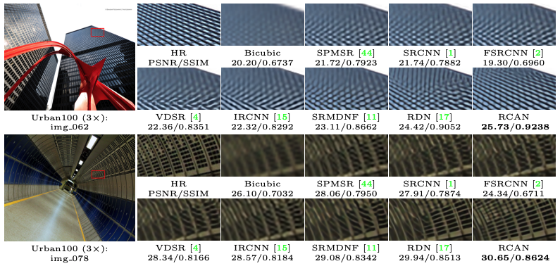
Figure 5. A comparison between the results of RCAN and various other architectures. [2].
Residual Dense Networks (RDN)
The Residual Dense Network revolutionizes SR by addressing limitations in prior architectures such as SRDenseNet and MemNet. By fully utilizing hierarchical features, RDN achieves state-of-the-art performance.The introduction of RDBs ensures efficient feature reuse, while LFF stabilizes training and adapts to varying feature scales. This design allows RDN to extract and combine multi-level features effectively. The GFF module distinguishes RDN by adaptively combining features from all RDBs. This approach enhances the network’s ability to capture intricate details across multiple levels, resulting in sharper and more realistic HR images. With its modular design, RDN scales efficiently across different upscaling factors (×2×2×2, ×3×3×3, ×4×4×4), outperforming traditional methods in tasks requiring high-quality image restoration.
Key Concepts
- Residual Dense Blocks (RDBs): These are the foundational building blocks of RDN. Each RDB incorporates dense connectivity, ensuring that every convolutional layer has direct access to the output of all previous layers. This dense connectivity allows the network to fully utilize hierarchical features and improve feature reuse.
- Local Feature Fusion (LFF): Within each RDB, LFF is applied using a 1×1 convolutional layer. This mechanism adaptively combines feature maps, stabilizing training and enabling larger growth rates in the network.
- Global Feature Fusion (GFF): After passing through the RDBs, GFF integrates features from all residual dense blocks, ensuring that global hierarchical features are adaptively preserved.
- Contiguous Memory Mechanism (CM): Information from preceding RDBs is passed to all subsequent layers, facilitating a smooth flow of gradients and information throughout the network.
Architecture
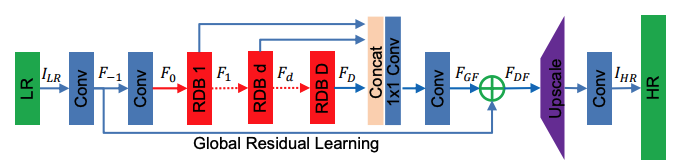
Figure 6. The RDN architecture. [1]. RDN employs a systematic approach to extract and utilize features for SR:
- Shallow Feature Extraction: The LR input image is processed through two convolutional layers. The first extracts basic features (F−1F_{-1}F−1), while the second (F0F_0F0) prepares the input for the dense feature extraction process.
- Residual Dense Blocks (RDBs): Each RDB consists of:
- Dense Connections: Every convolutional layer is directly connected to all other layers in the block.
- Local Feature Fusion (LFF): Combines feature maps from the current RDB and preceding layers, reducing the number of features via 1×1 convolution.
- Local Residual Learning (LRL): Improves the flow of information and gradients within the block.
- Global Feature Fusion (GFF): Outputs from all RDBs are combined, ensuring that global hierarchical features are fully utilized. The GFF step is critical for extracting features at multiple levels of abstraction.
- Upsampling Network (UPNet): Uses a pixel shuffle (sub-pixel convolution) layer to upscale the fused features to high resolution. The final HR image is reconstructed using a convolutional layer.
Key Results
| Dataset | Model | Bicubic | SPMSR | SRCNN | FSRCNN | VDSR | IRCNN_G | IRCNN_C | RDN | RDN+ |
|---|---|---|---|---|---|---|---|---|---|---|
| Set5 | BD | 28.78/0.8308 | 32.21/0.9001 | 32.05/0.8944 | 26.23/0.8124 | 33.25/0.9150 | 33.38/0.9182 | 33.17/0.9168 | 34.58/0.9280 | 34.70/0.9289 |
| DN | 24.01/0.5369 | -/- | 25.01/0.6950 | 24.18/0.6982 | 25.20/0.7183 | 25.70/0.7379 | 27.48/0.7597 | 28.47/0.8151 | 28.55/0.8173 | |
| Set14 | BD | 26.38/0.7271 | 28.89/0.8105 | 28.80/0.8074 | 24.44/0.7106 | 29.46/0.8244 | 29.63/0.8281 | 29.55/0.8254 | 30.53/0.8447 | 30.64/0.8463 |
| DN | 22.87/0.4724 | -/- | 23.78/0.5898 | 23.02/0.5856 | 24.00/0.6112 | 24.45/0.6305 | 25.92/0.6695 | 26.60/0.7101 | 26.67/0.7117 | |
| B100 | BD | 26.33/0.6918 | 28.13/0.7740 | 28.13/0.7736 | 24.86/0.6832 | 28.57/0.7893 | 28.65/0.7922 | 28.49/0.7886 | 29.23/0.8079 | 29.30/0.8093 |
| DN | 22.92/0.4449 | -/- | 23.76/0.5538 | 23.41/0.5567 | 24.00/0.5749 | 24.28/0.5900 | 25.55/0.6374 | 25.93/0.6573 | 25.97/0.6587 | |
| Urban100 | BD | 23.52/0.6862 | 25.84/0.7856 | 25.70/0.7770 | 22.04/0.6745 | 26.61/0.8136 | 26.77/0.8154 | 26.47/0.8081 | 28.46/0.8582 | 28.67/0.8612 |
| DN | 21.63/0.4687 | -/- | 21.90/0.5737 | 21.15/0.5666 | 22.22/0.6096 | 22.90/0.6429 | 23.79/0.7104 | 24.92/0.7364 | 25.05/0.7399 | |
| Manga109 | BD | 25.46/0.8149 | 29.64/0.9003 | 29.47/0.8924 | 23.04/0.7927 | 31.06/0.9234 | 31.15/0.9245 | 31.13/0.9234 | 33.97/0.9465 | 34.34/0.9483 |
| DN | 23.01/0.5381 | -/- | 23.75/0.7148 | 22.39/0.7171 | 24.20/0.7525 | 24.88/0.7765 | 26.07/0.8233 | 28.00/0.8591 | 28.18/0.8621 |
Table 2. Benchmark Results with BD and DN degradation models. Average PSNR/SSIM values for scaling factor x3. [3].
- PSNR (Set5 ×4): 32.47 dB
- SSIM (Set5 ×4): 0.8990
- These results highlight RDN’s effectiveness in recovering high-frequency details and textures in SR tasks. Compared to previous methods like SRCNN and MemNet, RDN demonstrates superior performance on diverse datasets.
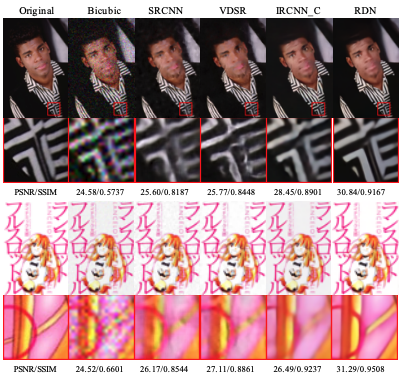
Figure 7. A prediction made by the RDN network. [3].
Implementing our Own Experiment
We’ve been working with the MiniPlaces dataset for the whole quarter, and the images in MiniPlaces are rather small (128x128), so we thought it would be an interesting experiment to perform super resolution on MiniPlaces to produce 256x256 outputs. Code
Approach
We decided to use the pre-trained models provided by the TorchSR library. These models are pre-trained on the Div2K dataset, which is very different from MiniPlaces. Therefore, we decided to fine-tune the models on MiniPlaces. To do this, we froze all of the pre-trained layers except for the upsampler modules, and used lr=1e-4 to fine-tune the upsampler module to learn features of MiniPlaces. We also decided to try using PSNR and SSIM as custom loss functions for the fine-tuning process.
Data Preprocessing
The MiniPlaces dataset contains images of size 128x128. The original 128x128 images are used as ground truths, so the training inputs are downscaled to 64x64.
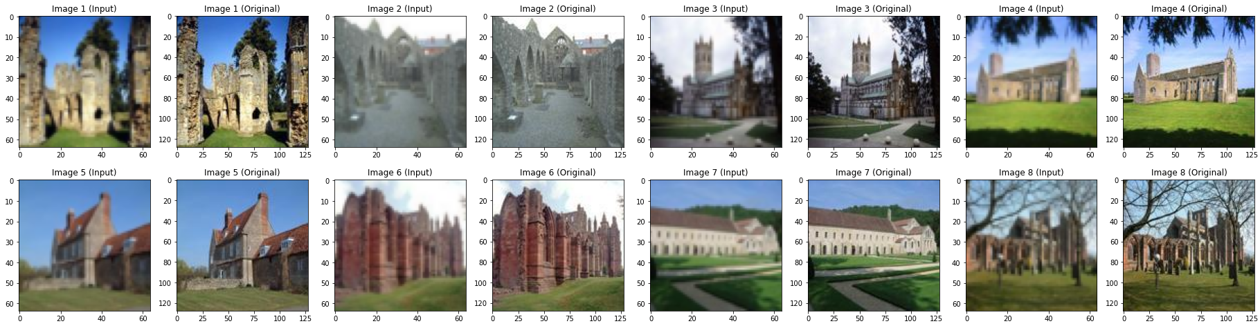
Figure 8. MiniPlaces images downscaled to 64x64, displayed side by side with the original 128x128 resolution.
Evaluation Metrics
We use PSNR and SSIM to evaluate the image metrics. PSNR is given by:
\[PSNR = 10 * \log_{10}\left(\frac{MAX_I}{MSE}\right)\]where \(MAX_I\) is the peak signal value in the image, in this case 1. SSIM is given by:
\[SSIM(x, y) = l(x,y)^{\alpha}c(x,y)^{\beta}s(x,y)^{\gamma}\]where \(x, y\) are pixel coordinates, \(l(x, y)\) is the luminance component at \((x, y)\), \(c(x, y)\) is the contrast component at \((x, y)\), \(s(x, y)\) is the structure component at \((x, y)\), and \(\alpha, \beta, \gamma\) are weights. We omit the derivations of the components for brevity, as they are not the focus of this section.
Training
We began by evaluating the pre-trained RCAN model on MiniPlaces. It achieved an average PSNR of 27.96 and average SSIM of 0.8921. The SR output is reasonable, but clearly has room for improvement.
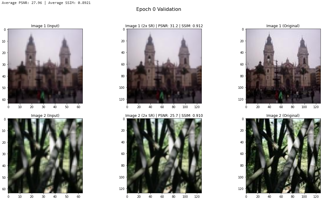
Figure 9. MiniPlaces epoch 0 validation output.
After 1 epoch of fine-tuning, we observed a substantial improvement on the validation set, with average PSNR climbing to 29.14 and average SSIM to 92.33. The SR output visually looks noticeably better.
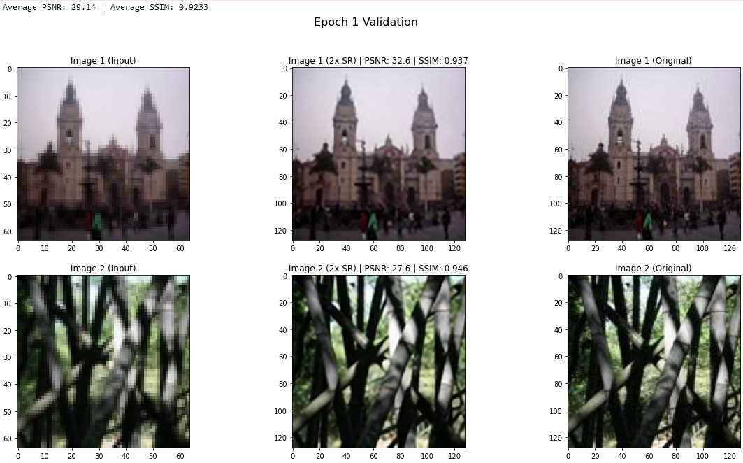
Figure 10. MiniPlaces epoch 1 validation output.
Further epochs did not produce meaningful improvements. We found that RCAN and EDSR achieved similar performance for this task, but decided to use RCAN because it trained considerably faster. SSIM as a loss function produced substantially better performance compared to PSNR or L1 loss.
Results and Reflection
Compared to the pre-trained RCAN, we observed that the fine-tuned model did produce sharper and more detailed 256x256 super resolution outputs. Due to a lack of ground truth images, we are unable to evaluate the test data more objectively than this.
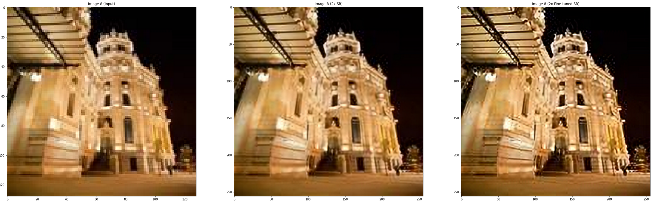
Figure 11. MiniPlaces test set output.
We are quite pleased with these results. A major limitation of performing super resolution on MiniPlaces is the low (128x128) resolution of the original images, which then has to be further downsampled to 64x64 to produce training data. There is not enough information present to produce extremely high quality super resolution outputs, so the noticeable improvement in quality can be considered a resounding success.
Overall Discussion and Future Work
The exploration of Enhanced Deep Residual Networks (EDSR), Residual Channel Attention Networks (RCAN), and Residual Dense Networks (RDN) reveals the evolving landscape of image super-resolution (SR) models driven by deep learning advancements. Each model introduces architectural innovations that address specific SR challenges while pushing the boundaries of reconstruction quality.
Strengths and Limitations
- EDSR: removal of batch normalization layers and use of residual scaling enable deeper networks with enhanced learning capacity. Its performance on standard datasets like Set5 and DIV2K is unparalleled. However, its computational demands make it less suitable for resource-constrained environments.
- RCAN: excels with its Residual-in-Residual (RIR) and Channel Attention (CA) mechanisms, which effectively capture high-frequency textures while maintaining stability during training. Despite its exceptional performance, the large number of layers can pose training challenges and increase memory consumption.
- RDN: dense feature extraction strategy, facilitated by Residual Dense Blocks (RDBs) and Global Feature Fusion (GFF), ensures superior feature reuse. Its main limitation lies in its architectural complexity, which can complicate deployment in real-time systems.
Future Research Directions
- Lightweight Architectures: Future models could explore efficient architectures that maintain high SR performance with reduced computational costs, making SR more accessible for mobile and edge devices.
- New Datasets: Expanding SR benchmarks beyond conventional datasets like DIV2K and Set5 could foster models that generalize better to real-world scenarios, including low-light and noisy conditions.
- Generalization and Robustness: Future research should focus on improving robustness across diverse datasets and creating models that adapt dynamically to changing input resolutions.
- Multi-Scale and Self-Supervised Learning: Integrating multi-scale learning and self-supervised approaches could enhance model versatility while reducing dependency on large labeled datasets.
Conclusion and Takeaways
The evolution of deep learning-based SR models has redefined how image restoration tasks are approached. EDSR, RCAN, and RDN each exemplify a unique path toward addressing SR challenges through innovative architectural designs. EDSR pushes depth and capacity limits, RCAN optimally balances attention mechanisms, and RDN excels with feature fusion strategies. The continuous development of these models highlights the trade-offs between accuracy, complexity, and computational efficiency. By leveraging lightweight designs, expanding datasets, and enhancing generalization capabilities, the next generation of SR models promises to extend SR’s reach into broader and more demanding applications.
References
[1] Lim, B., Son, S., Kim, H., Nah, S., & Lee, K. M. (2017). Enhanced Deep Residual Networks for Single Image Super-Resolution. arXiv:1707.02921.
[2] Zhang, Y., Li, K., Wang, L., Zhong, B., & Fu, Y. (2018). Image Super-Resolution Using Very Deep Residual Channel Attention Networks. arXiv:1807.02758
[3] Zhang, Y., Tian, Y., Kong, Y., Zhong, B., & Fu, Y. (2018). Residual Dense Network for Image Super-Resolution. arXiv:1802.08797