Occlusion Removal Using DesnowNet
Occlusion removal in computer vision restores images by addressing obstructions, including removing weather conditions such as rain, fog, snow, and haze. These weather-induced occlusions hinder object detection and thus can impact the performance of computer vision models. Deep learning-based techniques such as convolutional neural networks (CNNs) and generative adversarial networks (GANs) can be used to remove weather artifacts from image content. These models exploit spatial and temporal features, preserving key features of images while removing occlusions from the background. Applications range from autonomous driving to surveillance, where improved image clarity under challenging weather conditions enhances safety and accuracy. In our project, we attempt to create an implementation of DesnowNet. View our code here.
- 1. Introduction
- 2. Background and Related Work
- 2. Proposed Method
- 3. Dataset and Downscaling the Network
- 4. Results
- Reference
1. Introduction
The goal of this project is to explore the robustness and practicality of the occlusion removal architecture in a constrained environment with limited computing resources and a downscaled dataset. For this project, we decided to aim specifically at the architecture presented by the paper “DesnowNet: Context-Aware Deep Network for Snow Removal”. The purpose of the neural network is to remove the snow (noise) in snowy images and recover a snow-free image. The neural network is designed to remove snow (viewed as noise) from images and recover clear, snow-free visuals. While the original paper demonstrated strong results, we adapted the method to a scaled-down Snow100K dataset and evaluated its performance in a simplified setup.
Our work builds on the DesnowNet framework, focusing on understanding its ability to generalize under constraints. This includes analyzing the architecture’s modular components, adapting it for more efficient computation, and measuring performance on this reduced dataset. We also reflect on the challenges of balancing computational limits with maintaining model effectiveness. The rest of this paper is structured as follows:
2. Background and Related Work
Understanding Image Restoration
Image restoration is a fundamental task in computer vision that aims to recover high-quality images from degraded inputs. Degradation can occur due to various factors, including noise, motion blur, glare, or occlusions. This process is crucial for applications where clear and accurate visuals are required, and it often serves as a pre-processing step for downstream tasks like image classification, object detection, or scene understanding.
In traditional machine learning pipelines, image restoration tasks are handled by minimizing a loss function that quantifies the difference between the restored image and the ground truth. Modern methods leverage deep learning models to capture complex patterns of degradation and restoration, achieving state-of-the-art results across various tasks.

Fig 1. Example of a restored image [1].
Importance of Image Restoration
Image restoration is not just a theoretical exercise but has significant practical implications. The quality of restored images directly impacts the performance of subsequent tasks in various applications, such as:
- Autonomous Vehicles: Ensuring robust navigation and obstacle detection under challenging weather or lighting conditions.
- Security and Surveillance: Enhancing the clarity of surveillance footage for better monitoring and incident analysis.
- Photography and Media: Providing tools for professional and consumer-grade image enhancement.
- Scientific and Medical Imaging: Enabling accurate analysis of degraded images in fields like astronomy, radiology, and microscopy.
Restoring degraded images ensures that critical information is preserved and can be reliably analyzed, regardless of the domain.
Techniques in Image Restoration
Several specialized tasks fall under the umbrella of image restoration, each requiring unique methods and architectures:
- Denoising: Removing random noise introduced during image capture, such as sensor noise in low-light conditions.
- Deblurring: Correcting blur caused by motion, focus errors, or camera shake.
- Occlusion Removal: Addressing obstructions, such as rain streaks, snow, or dirt, that obscure parts of the image.
- Super-Resolution: Enhancing image resolution to reveal finer details, often beyond the original capture quality.
Traditional approaches to these problems often relied on hand-crafted features and assumptions about the degradation model (e.g., Gaussian noise for denoising). However, deep learning has revolutionized the field by enabling models to learn directly from data, resulting in more flexible and powerful solutions.
Image Restoration as a Step in the Vision Pipeline
Image restoration plays a pivotal role in the broader vision pipeline. It acts as the bridge between raw image capture and high-level computer vision tasks such as:
- Image Classification: Assigning labels to objects or scenes in an image.
- Object Detection: Identifying and localizing objects within an image.
- Semantic Segmentation: Understanding the pixel-wise classification of scenes.
For instance, degraded images can severely impact the accuracy of classification models, making restoration a critical pre-processing step. This pipeline—moving from image capture to restoration and then analysis—ensures robustness in practical systems like autonomous vehicles and security networks.
Deep Learning and Specialized Models
With the rise of deep learning, image restoration has evolved from task-specific models to modular architectures that can tackle multiple types of degradation. For example, models like convolutional neural networks (CNNs) and attention-based mechanisms have been adapted to handle specific challenges like translucency recovery and residual generation, as seen in architectures such as DesnowNet.
Despite their success, these models often face challenges in generalization and scalability, particularly when deployed in resource-constrained environments or with limited training data. Recent efforts in the field have focused on creating lightweight, adaptable architectures capable of maintaining performance under such constraints.
By combining these advancements with task-specific knowledge, modern image restoration methods continue to push the boundaries of what is possible, enabling more robust and versatile vision systems.
2. Proposed Method
The general mathematical equation is as follows:
\[x = a \odot z + y \odot (1 - z) \tag{1}\]Where:
\(x\) is the snowy color image, a combination of the snow-free image \(y\) and a snow mask \(z\). \(\odot\) denotes element-wise multiplication, and \(a\) represents the chromatic aberration map.

Fig 2. Overview of DesnowNet [1].
To estimate the snow-free image \(\hat{y}\) from a given \(x\), we must also estimate the snow mask \(\hat{z}\) and the aberration map \(a\). The original paper used a neural network with two modules:
- Translucency Recovery (TR)
- Residual Generation (RG)
The translucency recovery module focuses on representing the snow in the image as a mask and using this mask to remove the translucent snow artifacts to create an approximation of the snow-free image. The residual generation module is used to restore finer textures and details that were removed by the translucency recovery step.
The relationship between \(\hat{y}\) for residual generation is described as:
\[\hat{y} = y' + r \tag{2}\]2.1 Descriptor
Both TR and RG consist of Descriptor Extraction and Recovery submodules. This section will focus on the descriptor module. Descriptors are compact representations of features from an image and are extracted using an Inception-V4 network as a backbone and a subnetwork termed as the dilation pyramid (DP), defined as:
\[f_t = \gamma \|_{n=0}^{n} B_{2n} (\Phi(x)) \tag{3}\]Where:
- \(\Phi(x)\) represents the features from the last convolution layer of Inception-V4,
- \(B_{2n}\) denotes the dilated convolution with dilation factor \(2n\).
The Inception architecture is particularly suited for capturing multi-scale features due to its ability to process information across varying filter sizes within the same layer. The dilation pyramid applies dilated convolutions with varying dilation rates, enabling the network to capture spatial dependencies at multiple scales without increasing the number of parameters.
Our descriptor module was defined as follows.
class DescriptorT(nn.Module):
  def __init__(self):
    super(DescriptorT, self).__init__()
    self.iv4 = InceptionV4()
    self.dp  = DilationPyramid()

  def forward(self, x):
    out_iv4 = self.iv4(x)
    out     = self.dp(out_iv4)
    return out
Here is how InceptionV4 and DilationPyramid were initialized:
class InceptionV4(nn.Module):
    def __init__(self, in_chans=3, output_stride=32, drop_rate=0.):
        super(InceptionV4, self).__init__()
        self.drop_rate = drop_rate

        self.features = nn.Sequential(
            BasicConv2d(in_chans, 16, kernel_size=3, stride=1, padding=1),
            BasicConv2d(16, 16, kernel_size=3, stride=1, padding=1),
            BasicConv2d(16, 32//factor, kernel_size=3, stride=1, padding=1),
            Mixed3a(),
            Mixed4a(),
            Mixed5a(),
            InceptionA(),
            InceptionA(),
            InceptionA(),
            InceptionA(),
            ReductionA(),  # Mixed6a
            InceptionB(),
            InceptionB(),
            InceptionB(),
            InceptionB(),
            InceptionB(),
            InceptionB(),
            InceptionB(),
            ReductionB(),  # Mixed7a
            InceptionC(),
            InceptionC(),
            InceptionC(),
        )
class DilationPyramid(nn.Module):
  def __init__(self, gamma=4):
    super(DilationPyramid, self).__init__()
    self.dilatedConv0 = nn.Conv2d(768//factor, 384//factor, kernel_size=3, dilation=1, padding=1)
    self.dilatedConv1 = nn.Conv2d(768//factor, 384//factor, kernel_size=3, dilation=2, padding=2)
    self.dilatedConv2 = nn.Conv2d(768//factor, 384//factor, kernel_size=3, dilation=4, padding=4)
    self.dilatedConv3 = nn.Conv2d(768//factor, 384//factor, kernel_size=3, dilation=8, padding=8)
    self.dilatedConv4 = nn.Conv2d(768//factor, 384//factor, kernel_size=3, dilation=16, padding=16)
2.2 Recovery Submodule
The recovery submodule of the TR module generates the estimated snow-free image by recovering the details behind translucent snow particles. It consists of:
-
Snow mask estimation (SE): Generates a snow mask, which indicates the regions of the image affected by snow. The snow mask acts as a map where each pixel represents the amount of snow occlusion, with values closer to 1 representing areas with a lot of snow and values closer to 0 representing snow-free regions \(\hat{z}\).
-
Aberration estimation (AE): Generates the chromatic aberration map for each RGB channel. Chromatic aberration occurs when snow particles distort the color and brightness of the image by scattering light.
A new architecture, termed Pyramid Maxout, is used to select robust feature maps. The Pyramid Maxout architecture is effective in handling complex snow patterns because it combines features from multiple receptive fields:
\[M_{\beta}(f_t) = \text{max}( \text{conv}_1(f_t), \text{conv}_3(f_t), \dots, \text{conv}_{2\beta-1}(f_t) ) \tag{4}\]The TR module recovers the content behind snow:
\[y'_i = \begin{cases} \frac{x_i - a_i \times \hat{z}_i}{1 - \hat{z}_i}, & \text{if } \hat{z}_i < 1 \\ x_i, & \text{if } \hat{z}_i = 1 \end{cases} \tag{5}\]The RG module complements the residual \(r\) for improved image reconstruction:
\[r = R_r(D_r(f_c)) = \sum_{\beta} \text{conv}_{2n-1}(f_r) \tag{6}\]Here are the definitions of the aforementioned modules:
class PyramidMaxout(nn.Module):
  def __init__(self, out_dim=None):
    super(PyramidMaxout, self).__init__()
    self.conv1 = nn.Conv2d(1920//factor, out_dim, kernel_size=1)
    self.conv3 = nn.Conv2d(1920//factor, out_dim, kernel_size=3, padding=1)
    self.conv5 = nn.Conv2d(1920//factor, out_dim, kernel_size=5, padding=2)
    self.conv7 = nn.Conv2d(1920//factor, out_dim, kernel_size=7, padding=3)

class SnowExtractor(nn.Module):
  def __init__(self):
    super(SnowExtractor, self).__init__()
    self.pyramidMaxout = PyramidMaxout(out_dim=1)
    self.prelu = nn.PReLU()


class AberrationExtractor(nn.Module):
  def __init__(self):
    super(AberrationExtractor, self).__init__()
    self.pyramidMaxout = PyramidMaxout(out_dim=3)
    self.prelu = nn.PReLU()

class PyramidSum(nn.Module):
  def __init__(self,out_dim=None):
    super(PyramidSum, self).__init__()
    self.conv1 = nn.Conv2d(1920//factor, out_dim, kernel_size=1)
    self.conv3 = nn.Conv2d(1920//factor, out_dim, kernel_size=3, padding=1)
    self.conv5 = nn.Conv2d(1920//factor, out_dim, kernel_size=5, padding=2)
    self.conv7 = nn.Conv2d(1920//factor, out_dim, kernel_size=7, padding=3)

class RecoveryR(nn.Module):
  def __init__(self):
    super(RecoveryR, self).__init__()
    self.pyramidSum = PyramidSum(out_dim=3)
2.3 Loss Function
A loss network is constructed to measure losses at certain layers:
\[L(m, \hat{m}) = \sum_{\tau=0}^{\tau} \| P_{2i}(m) - P_{2i}(\hat{m}) \|_2^2 \tag{7}\]The overall loss function is defined as:
\[L_{\text{overall}} = L_{y'} + L_{\hat{y}} + \lambda_{\hat{z}} L_{\hat{z}} + \lambda_w \| w \|_2^2 \tag{8}\]Where:
- \(L_{\hat{z}} = L(z, \hat{z})\),
- \(L_{\hat{y}} = L(y, \hat{y})\),
- \(L_{y'} = L(y, y')\).
Here is our final network architecture and implementation of our loss function:
class DeSnowNet(nn.Module):
  def __init__(self):
    super(DeSnowNet, self).__init__()
    self.descriptorT    = DescriptorT()
    self.snowExtractor  = SnowExtractor()
    self.aberrationExtractor = AberrationExtractor()

    self.descriptorR    = DescriptorR()
    self.recoveryR      = RecoveryR()

  def forward(self, x):
    f_t     = self.descriptorT(x)
    z_hat   = self.snowExtractor(f_t)
    a       = self.aberrationExtractor(f_t)
    y_prime  = self.recover(x, z_hat, a)
    f_c     = torch.cat((y_dash, z_hat, a), 1)

    f_r     = self.descriptorR(f_c)
    r       = self.recoveryR(f_r)

    y_hat   = torch.add(y_prime, r)

    return y_hat, y_prime, z_hat

  def recover(self, x, z_hat, a):
    mask = z_hat<1.0
    out = (x-(a*z_hat))/(1-z_hat)
    out = out*mask+x*(~mask)
    return out
class DeSnowNetLoss(nn.Module):
  def __init__(self, lambda_z, t):
    super(DeSnowNetLoss, self).__init__()
    self.lambda_z = lambda_z
    self.t = t

  def forward(self, y_original, z_original, y_dash, y_hat, z_hat):
    Loss_y_prime  = self.pyramidLoss(y_original, y_dash, self.t)
    Loss_y_hat   = self.pyramidLoss(y_original, y_hat, self.t)
    Loss_z_hat   = self.pyramidLoss(z_original, z_hat, self.t)
    Loss_overall = Loss_y_prime + L_y_hat + (self.lambda_z * L_z_hat)
    return L_overall

  # Pyramid Loss
  def pyramidLoss(self, m, m_hat, t):
    loss = 0
    for i in range(t):
      k = pow(2,i)
      poolM     = nn.MaxPool2d(kernel_size=(k,k), stride=(k,k))
      poolM_hat = nn.MaxPool2d(kernel_size=(k,k), stride=(k,k))
      t1 = poolM(m)
      t2 = poolM_hat(m_hat)
      diff = torch.sub(t1, t2)
      diff = torch.square(diff)
      sums = torch.sum(diff)
      loss += sums
    return loss
3. Dataset and Downscaling the Network
Due to limited computing resources and storage, a downscaled version of the Snow100K dataset was used, consisting of 10,000 images. The original neural network architecture was also scaled down by a factor of 2 to enable training on Google Colab. Training was stabilized with a smaller number of epochs.
4. Results
Despite downscaling the network and dataset, the performance was acceptable. Though not perfect, most of the smaller specks of snow were removed or greatly faded. For bigger patches of snow, our model faded them a bit but they still remained obvious in the image.
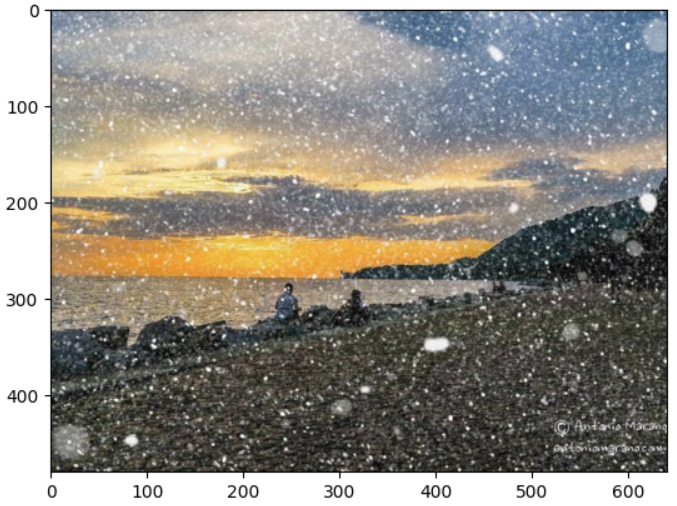
Fig 3. Original image with lots of synthetic snow [2].
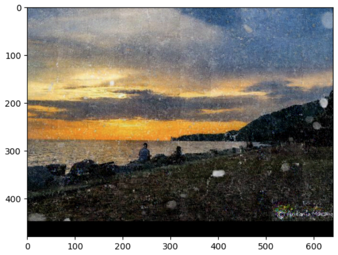
Fig 4. Corresponding output image of our DesnowNet model [3].
Reference
[1] Liu, Yun-Fu, et al. “DesnowNet: Context-Aware Deep Network for Snow Removal” https://doi.org/10.48550/arXiv.1708.04512. 2017.
[2] Fu, Xueyang, et al. “Clearing the Skies: A deep network architecture for single-image rain removal” https://doi.org/10.48550/arXiv.1609.02087. 2016.
[3] Valanarasu, Jeya, et al. “TransWeather: Transformer-based Restoration of Images Degraded by Adverse Weather Conditions.” https://doi.org/10.48550/arXiv.2111.14813. 2021.