Optical Flow
Optical flow is simply the problem of estimating motion in images, with real world applications in other fields such as autonomous driving. As such, there have been many different approaches to this problem. We compare three of these approaches: FlowNet, RAFT, and UFlow. We explore each of these models in depth, before moving on to a comparative analysis and discussion of the three models. This analysis highlights the key differences between each approach, when they are most applicable, and how they each handle common problems in the optical flow field such as the lack of available training data.
- 1. Introduction
- 2. Background & Timeline
- 3. FlowNet: Pioneering Deep Learning for Optical Flow
- 4. RAFT: Optical Flow Models and Training Techniques in Data-Constrained Environment
- 5. UFlow: What Matters in Unsupervised Optical Flow
- 6. Comparative Analysis
- 7. Discussion
- 8. Conclusion
- Reference
1. Introduction
The problem of optical flow in computer vision is simply the estimation motion in images, represented as a flow field at the pixel level. Being able to effectively solve this problem is crucial to many real-world applications, such as autonomous driving, object tracking, and general robotics. While the problem statement may be simple, there are various factors which make this a challenging task in practice. As such, the problem of optical flow is a fundamental one in the field of computer vision.
Given how complex the issue of optical flow is, there have been many different attempts, spanning multiple machine learning paradigms, in an attempt to solve it. Traditionally, researchers in this field have taken a supervised learning approach, commonly with convolutional neural networks, to solve this problem. Most notably, the FlowNet model, along with the RAFT architecture, are among the state of the art in optical flow supervised learning. However, the unsupervised learning approach has recently gained traction in this field, largely driven by a global issue in optical flow problem, which is a lack of labeled training data. In fact, the magnitude of this issue is so great that supervised approaches often rely on synthetic data to train the models. Among unsupervised learning models, UFlow is the most notable.
The scope of this report is to take a deep dive into each of these approaches. This is accomplished by first exploring each of these models individually, and then completing an analysis of how they compare. The individual descriptions include the relevant architectures, training methodologies, and other uniqueness factors. The final analysis and discussion will not only display the strengths and weaknesses of each approach, but also provide a timeline for how this field has progressed over time. The benchmarks and datasets used to compare these approaches are the standards in the optical flow field, including the endpoint error metric and the Sintel and KITTI datasets. Further, the applicable use cases for each of these approaches will also be discussed.
2. Background & Timeline
Progress and Breakthrough
Prior to the deep learning era, optical flow estimation, which calculates a pixel-wise displacement field between two images , was initially formulated as a continuous optimization problem. The foundational work in this domain was done by Horn and Schunck. Later methods, like DeepFlow (2013), blended classical techniques such as a matching algorithm (that correlates multi-scale patches) with a variational approach to better handle large displacements.
In the era of DL, it showed it could bypass the need to formulate an explicit optimization problem and train a network to directly predict flow. This revolution began with FlowNet (2015), the first CNN model to solve optical flow as a supervised learning task. FlowNet used a generic CNN architecture with an added layer that represented the correlation between feature vectors. Following this, models like FlowNet2 (2017) improved performance by stacking multiple FlowNet architectures but required a large number of parameters (over 160M). This led to a subsequent focus on creating smaller, more efficient models, such as SpyNet (2016), which was 96% smaller than FlowNet , and PWC-Net (2018), which was 18 times smaller than FlowNet2. The current state-of-the-art model is RAFT (Recurrent All-Pairs Field Transforms) (2020), which combines CNN and RNN architectures, updates a single high-resolution flow field iteratively, and ties weights across iterations.
Datasets
Optical flow models heavily utilize large, synthetically generated datasets. Key benchmarks include: KITTI 2015, which comprises dynamic street scenes captured by autonomous vehicles; MPI Sintel, derived from a 3D animated film, which provides dense ground truth for long sequences with large motions; and the purely synthetic datasets Flying Chairs and Flying Things3D, which trade realism for quantity and arbitrary amounts of samples.
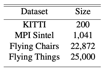
Figure 1. KITTI is the only non-synthetic dataset. Its size compared to other synthetic datasets highlights the scarcity of real-world data [2].
Scarcity of Real-world Data
One of the core limitations in optical flow research is the difficulty of collecting real-world optical flow ground truth data. Due to this, the domain lacks any large, supervised real-world datasets. Optical flow models often have to rely on synthetic data, which are simulated by computers. However, this data is too “clean’, in which it doesn’t have the natural artifacts that real-world data has such as motion blur, noise, etc. Because of this, models trained on synthetic data alone may not be well-equipped to handle the noisy data in real life. Later on, we will discuss an alternative to supervised learning as a way to combat this data scarcity problem.
3. FlowNet: Pioneering Deep Learning for Optical Flow
FlowNet Motivation
CNNs had been succesful in recognition/classification tasks by 2015, but optical flow estimation had never been succesfully by way of CNNs. A reason for this is becuase optical flow is particularly challenging, as it requires precise per-pixel localization and finding corresponses between two images. This means that the network must learn image feature representations and learn to match them at different locations at the same time, which is not something that CNNs had been used for prior to FlowNet. Before this, variational approaches, like Horn and Schunk, dominated the field of optimal flow, but required handcrafted features and manual paremeter tuning. Like mentioned earlier, one huge obstacle for making a CNN optical flow model is the fact that existing datasets that could be used to train these models were far too small to get anything meaningful, with the largest optical flow dataset being Sintel, with only 1041 pairs of images. However, the creation of the synthetic Flying Chairs dataset, with ~23,000 image pairings, gave way to much more exploration of optical flow models using a CNN architecture.
In short, the FlowNet model uses a CNN to take 2 input images, usually a before position and after position, and predict the optical flow field, which represents where each pixel has moved to from the first image to the second image.
Architecture Overview
At a high level, FlowNet is built using an encoder-decoder structure, with information being spacially compressed in the contractive portion first, then refined in the expansion portion, with layers on top of this convolutional portion that are used to actually predict the optical flow field based on the features produced by the convolutional network.
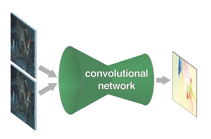
Figure 2. High level picture of the FlowNet Architecture [1].
In the contractive portion, there are 9 covolution layers total, 6 of them using a stride of 2 to act as a pooling mechanism. Each of them contain a ReLU activation to introduce non-linearity. In these 9 layers, there are no fully-connected layers, allowing for images of any size.
In the expanding portion, FlowNet uses “upconvulitional” layers, which performs unpooling followed by convolution. Upconvolved feature maps are then concatenated with corresponding feature maps from the contractive portion, which helps preserve high level info and lower level details from deeper within the network. This “upconvolution” process is repeated 4 times, doubling the resolution each step. The final output is at 1/4 the size of the input resolution, then uses bilinear upsamling in order to get the full resolution.
FlowNetSimple vs FlowNetCorrelated
FlowNet actually has two seperate models, both with their own strengths.
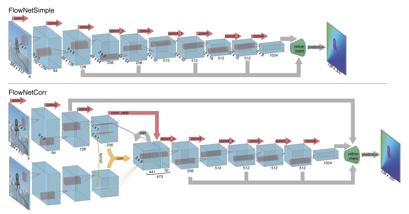
Figure 3. Comparison between FlowNetSimple vs. FlowNetCorrelated architectures [1].
In FlowNetSimple, both images are just stacked together along the channel dimension, and fed through the generic convolutional network. Because of this, the network has complete freedom on to learn how to process the pair of images, with no constraints on the internal representations on matching strategies.
In FlowNetCorr, on the other hand, the two input images are processed through seperate but identical convolutional streams, and those streams produce independent feature representations for each image. Then, the individual representations are combined through a specialized correlation layer, which is used to determine the similarity between portions of the two images. After this, FlowNetCorr goes back to the traditional FlowNet approach by adding convolutional layers on top which is used to predict the flow mapping.
While we will analyze the results more shortly, at a high level FlowNetCorr performs better on simple data, like the Flying Chairs and Sintel Clean datasets, but has a tougher time with large displacemenets between photos and more noisy images, that maybe have motion blur or other things of that nature.
Training FlowNet
As mentioned beforehand, optical flow models are not the easiest to train, mainly due to the fact that ground truth data is hard to come by, and usually has to be simulated. Because of this, the Flying Chairs dataset was used as it had the most ground truth image pairings out of any dataset at the time, with around 23,000 different simulated pairings. Along with this simulated data to help train, there was also data augmentation which was used to diversify and not overfit to the simple, clean images that are within the Flying Chairs dataset. Augmentation techniques included simple geometric transformations like translation, rotating, and scaling, as well as additive Gaussian noise features like brightness, contrast, gamma, and color.
In terms the actual loss function, endpoint error (EPE) is used, which is measured as the euclidean distance between the predicted flow vector and the ground truth movement of pixels, averaged over all pixels.
\[\text{EPE} = \sqrt{(\Delta x_{gt} - \Delta x_{pred})^{2} + (\Delta y_{gt} - \Delta y_{pred})^{2}}\]Along with augmentation, finetuning can also be used to expand to other types of data, usualy more realistic datasets that wouldn’t normally contain enough data to train a whole model on.
Results
Like just mentioned above, FlowNet accuracy is based on the metric of EPE, which at a high level tells us how close average pixel in the predicted flow vector was to its ground truth flow vector.
FlowNet was evaluated on many different datasets with many options, but a table with a good representation of its strengths and limitations is listed here.
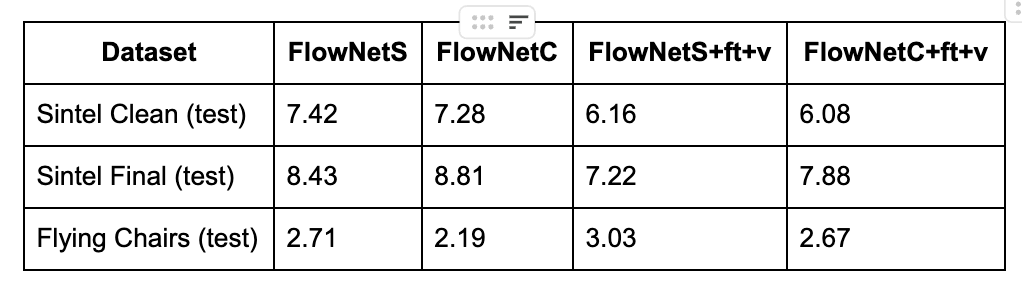
Figure 4. Evaluation Metrics on different datasets and FlowNet model options [1].
The different options used in evaluating FlowNet were +v and +ft, which correspond to the variatonal refinement and finetuning options respectively.
FlowNet models are trained on the Flying Chairs dataset. Because of this, the test EPE on this dataset was extremely low for all models, with a high of 3.03. As mentioned before, the FlowNetC model performs best on simple datasets, which was why it was able to achieve the lowest EPE out of all models and datasets with an EPE of only 2.19, compared to FlowNetS which achieved a 2.71 EPE. One thing that is interesting, however, is that the FlowNetS and FlowNetC actually perform worse with variational refinement and finetuning. This is because as the models were already trained on Flying Chairs, they have already learned the optimal representation for that specific data. Adding variational refinement (to smooth a noisy output in post-processing) and finetuning (which is done with the Sintel dataset) actually makes the model perform worse.
On the other datasets, Sintel Clean and Sintel Final, we can see the model performs significantly worse than on the Flying Chairs dataset, which makes sense for two reasons. One, the model is trained using Flying Chairs, but also Sintel is a more realistic dataset than Flying Chairs, so it is harder to capture all features correctly.
It can be seen in the Sintel Clean and Sintel Final results that FlowNetS performs better on a more noisy dataset (Sintel Final), where FlowNetC performs better on a cleaner dataset (Flying Chairs and Sintel Clean). As the finetuning was done on Sintel, we also see performance boosts from using it when evaluating on the Sintel datasets. Variatonal refinement also helped with these datasets, as it helps smooth the output (flow fields), as they are more noisy than the clean outputs from Flying Chairs that the model was trained on.
All in all, FlowNet performs very well compared to previous techniques that were used in optical flow, and has multiple options in practice which allow for a lot of flexibility in the datasets that it can process, without losing too much performance-wise. It’s options of FlowNetS and FlowNetC, along with variational refinement and finetuning allow for processing clean and noisy datasets effectively, and was a major breakthrough in terms of laying out a groundwork for using CNNs in optical flow going forward. Becuase of its success, there were many different models explored afterwards that are based on FlowNet, including RAFT, which will be explored next.
4. RAFT: Optical Flow Models and Training Techniques in Data-Constrained Environment
RAFT
RAFT (Recurrent All-Pairs Field Transforms) is a state-of-the-art optical flow model that combines CNN and RNN architectures. It consists of three main components:
-
A feature encoder that generates per-pixel feature vectors for both images, along with a context encoder that processes only the first image ($img_1$).
-
A correlation layer that constructs a 4D correlation volume by taking inner products between all feature pairs, then applies pooling to create multi-scale, lower resolution volumes.
-
A recurrent GRU-based update operator that starts with a zero flow field and iteratively refines it through repeated updates.
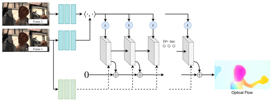
Figure 5. RAFT model architecture illustrating the feature encoder, correlation volume construction, and recurrent update operator [2].
Loss Function
The total loss ($L$) for RAFT-S is defined as the sum of losses on each recurrent block output. This is because the recurrent cell outputs create a sequence of optical flow predictions ($f_1, …, f_N$).
-
Distance Metric: The loss function for each output is the L1 distance between the ground truth ($gt$) and the upsampled prediction ($f_i$). This is the same distance metric used in the FlowNet loss function.
-
Weighting: The loss for each step in the sequence is weighted by an exponentially decreasing parameter, $\gamma$, where $\gamma=0.8$. This weighting gives more importance to earlier predictions in the sequence.
The total loss is expressed by the following formula:
\[L=\sum_{i=1}^{N}\gamma^{i-N}||gt-f_{i}||_{1} \text{, } \gamma=0.8\]One major design shift in RAFT is that it keeps a single high-resolution flow field and refines it directly, avoiding the usual coarse-to-fine upsampling strategy seen in earlier models. Its update module is a lightweight recurrent block that reuses the same weights across steps. For efficiency, RAFT-S was used, a smaller variant that reduces parameters by using narrower feature channels, slimmer bottleneck residual units, and a single $3\times3$ convolution GRU cell.
FlowNet Modification (Deconvolutional Upsampling)
DU was introduced as an alternative to the usual last stages of FlowNet, where the decoder output normally goes through another convolution and then a bilinear upsampling step. Instead, it uses a single transposed convolution to both learn richer features and scale the output, aiming to produce flow predictions that are more detailed and accurate.
Data Augmentations Used
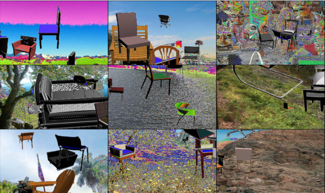
A set of augmentation methods was applied to the synthetic Flying Chairs dataset to help prevent overfitting, even though the dataset is already quite large. The hyperparameters followed those used for the original RAFT training setup, and the flow labels were adjusted after each transformation.
The methods used included:
- Cropping all images to the same size then normalize the pixel values.
- Random horizontal and vertical flips.
- Random stretching to simulate zooming in or out.
- Random asymmetric jitter, which alters brightness, contrast, saturation and hue.
- Random erasing of certain regions in the second image ($img_2$) of each pair.
| Flying Chairs before augmentation | Flying Chairs after augmentation |
|---|---|
 |
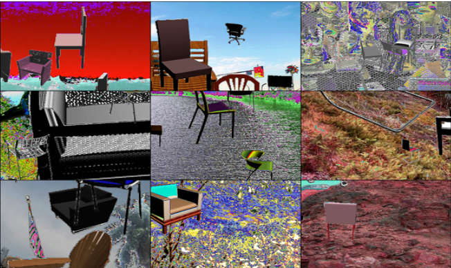 |
Figure 6. Visualization of Flying Chairs samples before and after data augmentation, showing the effects of geometric and photometric transformations used during training [2].
Evaluation Metrics
The primary metric was End-Point Error (EPE), which measures the Euclidean distance between the predicted flow vector and the ground-truth vector at each pixel:
\[\text{EPE} = \sqrt{(\Delta x_{gt} - \Delta x_{pred})^{2} + (\Delta y_{gt} - \Delta y_{pred})^{2}}\]Lower EPE values indicate more accurate flow estimates. We also report the percentage of pixels with errors below 1, 3, and 5 pixels (1px, 3px, 5px), which helps measure how well the model handles both small and moderate motions. Finally, we include the F1 outlier rate, defined as the percentage of pixels whose EPE exceeds both 3 pixels and 50% of the magnitude of the ground-truth flow. These metrics together allow us to compare overall accuracy, motion sensitivity, and robustness to outliers before analyzing model performance.
Results
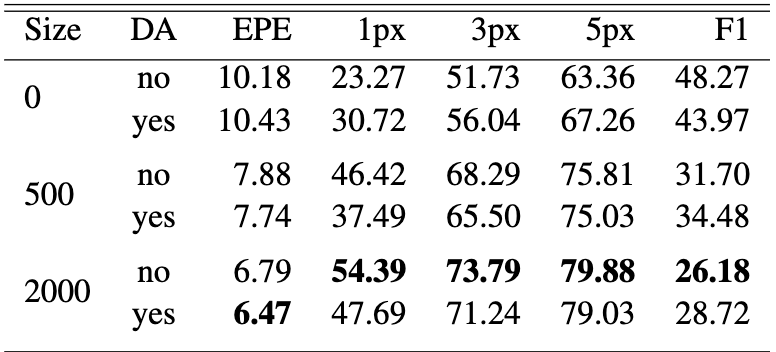
The experiments compared FlowNet, the modified FlowNet with deconvolutional upsampling (DU), and RAFT-S across different amounts of pre-training data (0, 500, and 2000 Flying Chairs pairs) and with or without data augmentation. All models were fine-tuned on 520 Sintel image pairs and evaluated on both Sintel and KITTI. Overall, the results showed that dataset size and augmentation played a major role in model performance, especially in low-data settings, and that RAFT benefited significantly more from augmentations than FlowNet.
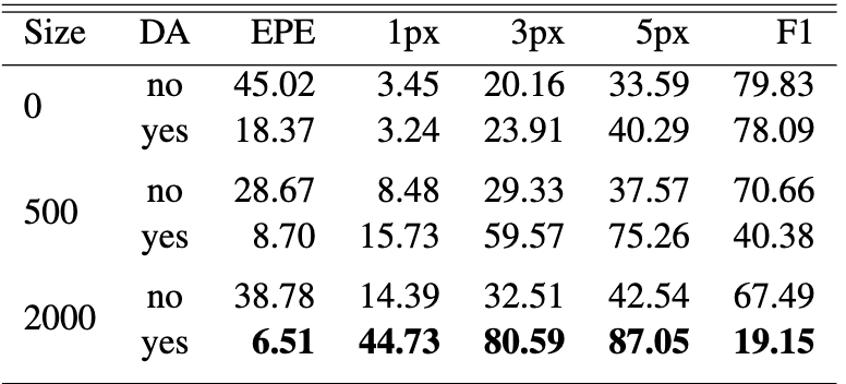
Across nearly all settings, increasing the number of Flying Chairs samples improved performance. On Sintel, FlowNet’s EPE dropped from 10.18 → 6.79 as pre-training rose from 0 to 2000 samples, and RAFT showed an even steeper improvement, especially when paired with augmentation (e.g., EPE 18.37 → 6.51 at 2000 samples). However, results on KITTI revealed that FlowNet did not always benefit from larger synthetic datasets, likely due to the domain gap between Flying Chairs and real scenes in KITTI, suggesting that mismatched pre-training can sometimes hurt generalization.
| Flownet on Sintel | Flownet on KITTI |
|---|---|
 |
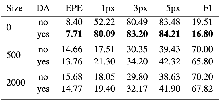 |
Figure 7. FlowNet performance on Sintel and KITTI, displaying metrics after fine-tuning under different data conditions [2].
Data augmentation consistently helped when the test domain differed from the training domain. For RAFT in particular, augmentation sharply reduced error. For example, on Sintel with 2000 pre-training samples, EPE improved from 38.78 (no aug) to 6.51 (with aug). FlowNet saw smaller gains, and in some Sintel cases the improvement was minimal, showing that FlowNet tends to overfit more regardless of augmentation.
| RAFT on Sintel | RAFT on KITTI |
|---|---|
 |
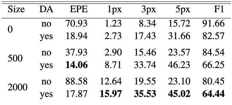 |
Figure 8. RAFT performance on Sintel and KITTI, displaying metrics after fine-tuning under different data conditions [2].
The modified FlowNet architecture with deconvolutional upsampling performed almost identically to the original. For instance, at 2000 pre-training samples on Sintel, the new model achieved an EPE of 6.80, essentially the same as the original 6.79. The only noticeable pattern was that DU gave a slight advantage when little or no pre-training data was available, while the original FlowNet recovered a small edge with larger datasets. Overall, the architecture change did not introduce meaningful improvements.
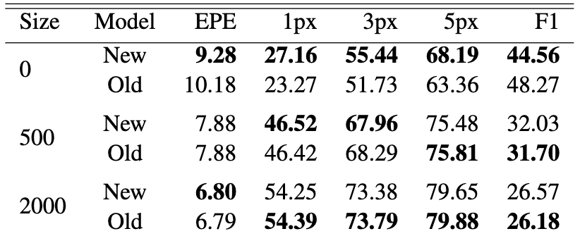
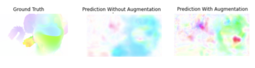
Figure 9. Predictions from the modified FlowNet model using deconvolutional upsampling, compared against the original architecture on Sintel [2].
Qualitatively, RAFT produced cleaner and more consistent flow fields than FlowNet, especially when pre-training and augmentation were combined. In scenes from the Driving and FlyingThings, RAFT captured fine-grained motion and global consistency better, while FlowNet focused more on object boundaries and sometimes missed motion details. In the low-data setting with no pre-training, RAFT still produced more coherent motion estimates, whereas FlowNet tended to rely heavily on edges rather than true frame-to-frame displacement.
| RAFT on Sintel (no pre-training) | Flownet on Sintel (no pre-training) |
|---|---|
 |
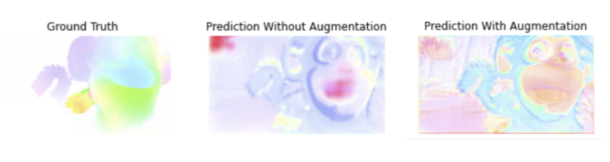 |
Figure 10. Comparison of RAFT and FlowNet without pre-training, illustrating RAFT’s stronger inductive bias for motion estimation in extremely low data conditions [2].
5. UFlow: What Matters in Unsupervised Optical Flow
Motivation: The Supervised Learning Bottleneck
One of the major limitations of supervised models attempting to solve the optical flow problem is the lack of available labeled data. As previously discussed, one approach to mitigating this issue is to generate synthetic data and use it to train the supervised models. While this can be a viable option, it is not without trade offs. Namely, this approach is less effective for objects with less rigid geometry, leading to manual intervention being needed [3].
Thus, an alternative solution to the optical flow problem is to abandon the supervised approach in favor of unsupervised models. This paradigm is particularly enticing because of how plentiful training data becomes, as any unlabeled video could be used. Additionally, unsupervised models typically showed advantages in inference speed and generalization as a result of being trained directly on real world (opposed to synthetic) data [3].
These reasons were the driving force behind the creation of the UFlow model, which was created as a means to determine the most important factors in training an unsupervised model. Among the aspects that were investigated were photometric loss, occlusion handling, and smoothness regularization.
Architecture & Training Components
The underlying architecture that UFlow is based on is the PWC-Net, which is then improved upon to determine the most important components. Because the pyramid, warping, and cost (PWC) approach was initially intended for supervised learning, adjustments had to be made during the creation of the UFlow model. For example, the highest pyramid level was removed to decrease the model size and dropout was incorporated for additional regularization.
Despite these changes, UFlow at its core uses a self-supervised training loop across five pyramid levels to ultimately predict the flow field from two images, as shown in the figure below. Firstly, a shared CNN is used to extract the features from the two images. These features are then fed into the pyramid, where each level has a loop involving warping, cost volume computation, and flow estimation. The warping layer in each block uses the current flow estimate to align the second image’s features with the first, creating the photo-consistency signal, which is needed to define photometric loss, the unsupervised training objective. The architecture behind the cost volume computation is a correlation layer, while the flow estimation at each block is done with a CNN.
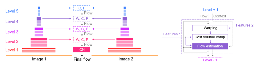
Figure 11. Overview of the UFlow model architecture, showing the pyramid structure as well as the WCF block present at each level [3].
As previously mentioned, the unsupervised training objective is the photometric loss. While the team behind UFlow experimented with multiple different losses, the main one used was the generalized Charbonnier loss function, given by
\[L_C = \frac{1}{n} \sum \left((I^{(1)} - w(I^{(2)}))^2 + \epsilon^2\right)^\alpha\]where \(\epsilon = 0.001\) and \(\alpha = 0.5\).
Ablation Studies: What Actually Matters?
With the base model established, the team behind UFlow aimed to determine exactly which components mattered the most in an unsupervised model for optical flow. The major components that were found to have the biggest effects following analysis were occlusion handling, data augmentation, and smoothness regularization.
Occlusion Handling
As previously mentioned, the UFlow model takes two images as input, and feeds them into a shared CNN for feature extraction. The issue of occlusions arises when specific features or regions of one image are not present in the partner image. If this is not accounted for and handled correctly, any photometric loss calculations would include garbage values. As such, all occlusions, along with any other pixels deemed invalid, need to somehow be detected and gracefully handled. The approach taken by UFlow is to use a “range map”, which stores information regarding the number of pixels in the partner image that are mapped to each pixel in a target image. This range map is then used to determine which pixels are not mapped to at all in the target image, and those pixels are deemed occlusions. Against the KITTI dataset specifically, the approach taken by UFlow is a forward-backward consistency check, which marks pixels as occlusions whenever the flow and back-projected flow disagree by more than some margin [3]. Thus, these pixels are “masked”. In this latter approach, the team found that stopping the gradient at the occlusion mask improved performance.
Data Augmentation Strategies
The next component that was analyzed within UFlow was data augmentation. Some of the data augmentation techniques used in training UFlow included color channel swapping, hue randomization, image flipping, and image cropping. However, the most emphasized augmentation technique during this process was continual self-supervision with image resizing. This specific method helped stabilize the training by starting with downsampled, lower-resolution images and then progressively increasing the input resolution over the training run, hence the resizing. The key result found by the team with respect to this factor was that both color and geometric augmentations were key for unsupervised models achieving good generalization.
Smoothness Regularization
In addition to data augmentation, one other component of UFlow that was analyzed was smoothness regularization. This aims to ensure that changes in flow estimations are not abrupt, which can happen for inputs with large homogenous regions. Specifically, the performance of both first-order and second-order smoothness regularization were investigated by the team. The difference between these two is simply which derivative of the estimated flow is being considered, and both can be represented by the equation below. The key finding related to this component was that it is significantly more beneficial to apply this smoothness regularization at the lower resolution of the flow itself opposed to the higher original input image resolution. In regards to the optimal regularization order, there was no answer as to which was definitely better, as the optimal order was different for the different datasets.
\[L_{\text{smooth}}^{(k)} = \frac{1}{n} \sum \exp\left(-\frac{\lambda}{3} \sum_{c} \left|\frac{\partial I_c^{(1,\ell)}}{\partial x}\right|\right) \left|\frac{\partial^k V^{(1,\ell)}}{\partial x^k}\right| + \exp\left(-\frac{\lambda}{3} \sum_{c} \left|\frac{\partial I_c^{(1,\ell)}}{\partial y}\right|\right) \left|\frac{\partial^k V^{(1,\ell)}}{\partial y^k}\right|\]where \(k\) denotes the order of smoothness (first-order or second-order), \(c\) indexes color channels, and \(\lambda\) controls the edge-aware weighting.
All together, a comparison of the estimated flow without each of these three components can be seen in the figure below.
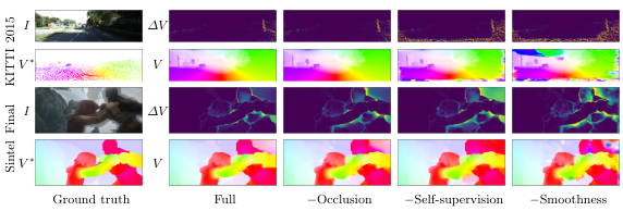
Figure 12. A visual comparison of how ablating each individual component, while holding the others constant, impacts the results. Examples from both KITTI and SINTEL shown. [3].
Results And Performance
In order to objectively determine which components of unsupervised models matter the most, the team had to quantitatively measure UFlow’s performance on multiple different datasets. The metrics used to benchmark the model were endpoint error and error rate, which are standard for the KITTI dataset and therefore the optical flow problem as a whole. In addition to KITTI, the Sintel dataset was also used to evaluate UFlow.
In terms of performance, the key takeaways were that UFlow set the new gold standard for unsupervised models, by performing at a similar level to the supervised FlowNet2, despite being completely trained without ground-truth labels. Of course, this was achieved through the careful evaluation, optimization, and combination of the various different components of an unsupervised model, and not a single new “breakthrough” technique.
Strengths & Limitations
Like any other engineering feat, the success of the UFlow model came with tradeoffs. One major strength of UFlow, and unsupervised learning as a whole in the optical flow problem, is the abundance of training data available for use. The ability to take any color video and train on it makes the unsupervised learning paradigm very appealing in the context of optical flow, especially considering the current lack of labeled data. Further, by training on real-world data opposed to almost exclusively synthetic data, UFlow has shown to achieve superior generalization on real-world inputs. Lastly, in the case of the UFlow model itself, there is clearly a systematic way of determining the importance of each of the major components, setting the foundation for future unsupervised learning models to tackle the optical flow problem.
However, UFlow did show that it has some limitations as well. Firstly, in the case of absolute performance, UFlow was still outperformed by the best fine-tuned supervised models (despite performing on par with popular supervised models like FlowNet2). Further, while it was previously discussed that each of the mentioned components can be tuned for optimal results, this tuning can be expensive in practice. This is because, in the process of training UFlow, the researching team had to train a new model for each ablation study. Lastly, in terms of hardware and physical requirements, the PWC-net used by UFlow can be memory intensive. As such, training an unsupervised model like UFlow typically requires more available memory.
6. Comparative Analysis
Supervised vs Unsupervised: Trade-offs
FlowNet: As FlowNet is a supervised approach, it requires a ground truth optical flow for training. However, the training requires there to be a mapping between every single pixel to its new matching pixel in the second image, meaning that it is very difficult to obtain real-world scenes, as the pixel correspondences cannot easily be determined. Because of this, FlowNet is typically trained on synthetic data, like the Flying Chairs dataset, as the images can be designed with the intent of mapping a pixel to another pixel in a second frame. So overall, a supervised learning approach scales really well and is able to learn easily by comparing its prediction to the ground truth, but the problem is that we don’t have the data in order to do so.
RAFT: RAFT operates entirely within the supervised setting, benefiting from accurate ground-truth labels that allow its recurrent refinement process to learn stable and precise motion estimates. This allows RAFT to consistently outperform earlier supervised models. However, RAFT inherits the major limitation of supervised learning: the scarcity of labeled optical flow data. As a result, it depends heavily on large-scale synthetic datasets such as Flying Chairs. While this strategy enables strong performance, it reduces flexibility compared to unsupervised models that can leverage real-world video.
UFlow: Being an unsupervised approach, UFlow is not susceptible to the same labeled data bottleneck as the supervised models. The tradeoff here is the added complexity in the training pipeline, as outlined in the ablation studies section.
Performance Comparison Across Datasets
FlowNet: According to the paper on FlowNet, “The endpoint error (EPE), which is the standard error measure for optical flow estimation. It is the Euclidean distance between the predicted flow vector and the ground truth, averaged over all pixels.” This is how the FlowNet Models were evaluated on different datasets, with the lower EPE value the better. All of these models did very well on the Flying Chairs dataset, likely because it is a simpler dataset and that is also what the models were trained on, and had a harder time with the Sintel dataset. The Sintel dataset was made of animated images, with the Clean dataset being ones that were just straight-forward images, and Final having tougher things like motion blur and other blemishes on the image that make it tougher to identify correlating pixels. However, in the models including +ft, we did see a slightly better performance. This makes sense as these models were finetuned with the Sintel dataset, compared to their counterparts (that didn’t include +ft) that had a worse performance, as they didn’t have the fine tuning. A main reason for the training being purely on the Flying Chairs dataset is because of how many samples are located within it, around 23,000, compared to Sintel which only contained around 1000 image pairings.
RAFT achieves high accuracy across benchmarks due to its dense correlation volume and iterative update operator. On Sintel, RAFT consistently outperforms FlowNet and produces significantly sharper flow predictions. Its performance does drop when trained with insufficient pre-training or augmentation, but once supplied with enough diversity, RAFT remains the strongest supervised model. On KITTI, domain shift limits its accuracy more noticeably, yet RAFT still surpasses FlowNet and remains competitive with top supervised methods.
UFlow: Uflow was evaluated on the field standard datasets KITTI and SINTEL. The final result was that UFlow could perform on par with supervised models such as FlowNet. However, when the supervised models were fine-tuned, they were able to achieve better performance than UFlow.
Training Data Requirements
FlowNet: One thing that makes it tough to have extremely accurate optical flow models is the lack of real-world ground truth data. Because of this, synthetic datasets are required in order to get enough data to train a supervised model. Like mentioned earlier, the FlowNet model is trained on the Flying Chairs synthetic dataset. This is for 2 reasons, one being its simplicity, but the other being the amount of data that is available. The 22,872 synthetic image pairs provide a decent amount of data for FlowNet to be trained on, compared to Sintel which only contains 1041 pairs. Another important feature of training the FlowNet model is data augmentation. These are making the images slightly different using translation, rotation, and scaling. This is just so the model doesn’t get too used to one specific POV and expect the chairs (and other items that will be evaluated) to all be the same size, shape, and orientation. This data augmentation proves to have a pretty significant impact on the EPE of its predictions, with about a 2 pixel increase in EPE on the Sintel dataset compared to training the model without it.
RAFT: RAFT’s architecture is powerful but data-hungry. With little or no pre-training, RAFT struggles to learn stable motion representations, resulting in high error. Performance improves rapidly as more Flying Chairs samples are added, and augmentation provides an even larger boost. This sensitivity highlights how much RAFT depends on both the quantity and variety of labeled or synthetic data. Compared to FlowNet, RAFT benefits more from scale but also degrades more sharply when data is scarce.
UFlow: Clearly, in terms of training data requirements, UFlow is the superior model. This is due to the fact that the unsupervised approach provides the model with an abundance of additional data to train on. As a direct result, the training process for UFlow does not require computational resources to be allocated to creating synthetic data, reducing the computational costs as well.
Generalization Capabilities
FlowNet: While it performs the best on the Flying Chairs dataset, as it was trained on it, the model does quite well on real-world data like Sintel and KITTI, with only a ~6 dropoff between the performance of EPE on Flying Chairs and Sintel, which when it comes down to it, is not a lot of displacement if we are speaking in terms of pixels. Along with a good overall generalization, the FlowNet model provides the FlowNetS and FlowNetC models, which can both be used for different types of datasets, depending on the need. FlowNetS takes the approach of literally just stacking the 2 images pixels on top of each other, to form an input of 6 values, RGB1 and RGB2. With this approach, the model basically just has to learn what every value means. And through its training, it will make inferences like, “The difference between R1 and R2 is important”, and other details of that nature. FlowNetC, on the other hand, basically instructs the model to compute how similar certain patches are. Basically, the model is told to compare one patch to other patches around it, and compare the similarities in order to determine which patch in the second image is the closest to the one being examined in the first image. Contrary to what many believed would be the case, FlowNetC is not better in all scenarios. It seems to do better when it comes to cleaner data, but actually performs worse than FlowNetS when it comes to challenging data. This is because FlowNetC somewhat overfits to the training data, while FlowNetS can infer some more complex relationships itself as it doesn’t have such rigid instructions.
RAFT generalizes better than earlier supervised models due to its strong inductive biases, yet it still faces challenges when moving from synthetic data to real-world scenes. On Sintel, RAFT adapts well with fine-tuning, but KITTI exposes limitations in matching the natural noise, lighting, and texture variations absent in synthetic pre-training. While RAFT is more robust than FlowNet, it cannot match the domain flexibility of unsupervised approaches like UFlow that learn directly from real imagery.
Generalization is one aspect where UFlow excels compared to other models. This is true even when the training and test data weren’t from the same domain. This is largely due to the fact that it is trained on real-world unlabeled data, which makes it more robust in practice.
Computational Costs
FlowNet: In the paper, the different FlowNet modes’ computation costs and times were evaluated using the NVIDIA GTX Titan GPU. FlowNetS and FlowNetC tend to be really fast when it comes to computation. On average, FlowNetS is able to process around 12.5 FPS, and around 6.7 FPS with FlowNet C. At a high level, FlowNetS would be able to process a 30 FPS video in only 2.4x the length of the original video. When the variational refinement option is used (+v), there is a large dropoff in the speed of the model. FlowNetS+v is about 12 times slower than its counterpart without the variational refinement option. However, the accuracy is proven to be better, but at a cost.
RAFT: RAFT’s accuracy comes with increased computation. Its all-pairs correlation volume and iterative GRU refinement make it more memory and computation intensive than FlowNet or PWC-Net. Inference is slower than FlowNet due to its complexity, though still feasible for many applications. RAFT represents a deliberate trade-off: higher computational requirements in exchange for better supervised accuracy.
UFlow: Recall that the UFlow architecture involves a PWC-Net, which progressively downsamples the input images. A direct result of this image resizing is reduced memory usage, which can be adjusted based on the number of levels used in the pyramid and how the images are resized.
Practical Considerations
FlowNet: In practice, FlowNet can be used in a variety of different ways, which makes it very attractive as a base model. It has extremely fast options like FlowNetS and FlowNetC, which both perform well on images with sharp edges and clear distinctions between items. For more challenging images, FlowNetS+v and FlowNetC+v can be used in order to trigger variational refinement to improve accuracy at the price of speed. The model is very adaptable, as it can take image inputs of any size with its fully convolutional nature, using a sliding window to parse images. It also doesn’t need hand-crafted features, as FlowNetS proves that it can take 2 RGB values from separate images and do an extremely good job of identifying patterns, even if images with more blemishes and blur. In all, FlowNet can be used in a variety of different ways for different use cases, and is a great model for other researchers to build their work off of.
RAFT: RAFT is a good choice when high accuracy is the priority and sufficient compute and synthetic training data are available. It excels in tasks that demand detailed motion estimation but is less suitable for low-resource environments or scenarios with extreme domain mismatch. RAFT also requires thoughtful data augmentation to reach peak performance. It is a high-performing but resource-intensive supervised model.
UFlow: As shown in the performance comparison, if absolute performance is the main objective, then finetuned supervised models outperform UFlow. However, in cases where domain-specific labeled training data is scarce, UFlow provides a good alternative which has proven to still perform on par with standard supervised models.
7. Discussion
Before FlowNet, classical variational approaches like Horn and Schunk dominated the optical flow field, no pun intended, for decades. These approaches relied heabily on handcrafted features and manually tuned parameters. FlowNet was the first model to demonstrate how CNNs could be used to learn optical flow directly from image pairs. Other models were built on top of this foundation, like RAFT, which used techniques like iterative refinement and dense correlation volumes, which allowed for a significant jump in accuracy over FlowNet. Along with these supervised techniques, UFlow also demonstrated how unsupervised learning can achieve similar accuracy scores, and opened a door to evaluate optical flow on real-world video data, which wasn’t the case beforehand.
These approaches all have their own strengths and weaknesses. First of all, FlowNet can be used when speed is a priorty. It achieves a very respectable accuracy on a variety of different types of data, and has options to prioritize speed vs accuracy, making it a very versatile option. RAFT should be used if accuracy is the top priority. It’s slower than FlowNet, requires more compute power, and a large set of synthetic training data, but also achieves the highest accuracy out of all models explored in this paper. Fine-tuning can also be used to achieve better performance on a target domain. UFlow, however, can be very valuable in a domain like optical flow. This is because ground truth data is harder to come by, and UFlow does not need this in order to perform well. It’s performance is on par with non-finetuned supervised model, and does extremely well with real-world videos, where syntehic data may not transfer well.
Going forward, the biggest thing that will improves model is the training data. Right now, there are synthetic datasets that do the job to a decent degree, but it would be largely beneficial to have bigger datasets that better match real-world distributions. Right now, the datasets are still on the small side, and don’t do a good enough job to represent real-world images. Aside from the training data, a more efficient iterative refinement in RAFT and the handling of larger displacements in FlowNet are key things that could improve the qualuty of the current models, as iterative refinement is quite slow, and FlowNet puts range limits on the correlation layers in exchange for performance, which inhibit FlowNetC’s capabilities. While there is much to be done, there are a large range of optical flow models out there currently, and a variety of different use cases that they fit into.
8. Conclusion
We discussed the evolution of the approaches to the optical flow problem over time, and analyzed the tradeoffs associated with the different approaches. We started by analyzing FlowNet, which acted as a pioneer for deep learning in the field of optical flow. The key point here was that FlowNet successfully used Convolutional Neural Networks to address the optical flow problem. Next was RAFT, which maintained the supervised approach, but used a feature encoder, correlation layer, and a recurrent GRU-based update operator as the key components in the solution. Lastly, we analyzed UFlow, which differed greatly from the other two models as UFlow was unsupervised. Comparing these three approaches did not reveal a definitive best model, but instead highlighted a different theme, which was that the optimization of the internal components of these models was more important than the exact training paradigm. This was also a key finding during the ablation studies from the team behind UFlow.
One theme that was apparent and common throughout the different approaches was that a lack of training data was a big motivator behind the methods used. As such, much of the realized success and innovations can be attributed to this one single constraint. For example, the RAFT model highlighted the importance of the data augmentation strategies used, a result achieved directly from the initial lack of sufficient labeled data. In the more extreme case, UFlow completely disregarded the need for labeled data and paired an unsupervised approach with research into which components were the most important. Once again, this innovation was driven from what was initially a major constraint. Clearly, this idea is extremely relevant in the optical flow field, but is also very generalizable to other fields of computer science, which may be currently limited by some constraint.
Clearly, the problem of optical flow is an important one, as there are many optical flow applications such as autonomous driving and robotics. As these fields grow, so will the need to find even better solutions to optical flow. The highlighted approaches show that there are multiple paths forward in this field, and future models will have the benefit of using the key findings from FlowNet, RAFT, and UFlow as the foundation.
Reference
Please make sure to cite properly in your work, for example:
[1] Fischer, Philipp, et al. “FlowNet: Learning Optical Flow with Convolutional Networks”. 2015.
[2] Isik, Senem, Shawn Zixuan Kang, and Zander Lack. “Optical Flow Models and Training Techniques in Data-Constrained Environment.” CS231N: Convolutional Neural Networks for Visual Recognition, Stanford University. 2022.
[3] Jonschkowski, Rico, et al. “What Matters in Unsupervised Optical Flow.” European Conference on Computer Vision (ECCV). 2020.