Self-Supervised Learning
Self-supervised Learning is a way for models to learn useful features without relying on labeled data. The model can create its own learning targets from the structure of the data. This method becomes popular in computer vision and many other fields because it makes use of large amounts of unlabeled data and can produce strong representations for downstream tasks. In this paper, we introduce the basic ideas behind self-supervised learning and discuss several common methods and why they are effective.
- Introduction
- Contrastive Learning (SimCLR)
- Masked Image Modelling (MAE)
- DINO: self-distillation with no labels
- Conclusion
- Reference
Introduction
Deep learning is a field that learns pattern and representations from data, and many of its breakthrough have relied on supervised learning. However, supervised learning depends on massive labeled datasets, and creating these labels is often expensive, time-consuming, and requires expertise. In many real situations, most datasets are unlabeled, which makes supervised learning difficult to apply in many practical situations. Therefore, self-supervised learning was developed to address this challenge. Instead of relying on human annotations, self-supervised learning creates pretext tasks that force the model to learn meaningful structure directly from the data itself.
Other than self-supervised learning, semi-supervised learning is also a useful way to train a model when labeled data is not sufficient. It uses both labeled and unlabeled data during training. In general, a semi-supervised learning workflow starts by training the model on the labeled data and then using the model’s own predictions to guide learning on the unlabeled data. Popular semi-supervised approaches include pseudo-labeling and consistency regularization. In practice, semi-supervised learning is preferred when at least some labels exist and we want to boost performance when adding unlabeled data. Self-supervised learning, on the other hand, is more suitable when obtaining labels is very difficult or expensive. In this paper, we will focus on several popular methods in self-supervised learning and discuss why they have become strong alternatives to fully supervised and semi-supervised approaches.
| Learning Method | Training Data |
|---|---|
| Supervised Learning | Fully labeled datasets |
| Self-Supervised Learning | Large-scale unlabeled datasets |
| Semi-Supervised Learning | Limited labeled data combined with large amounts of unlabeled data |
Contrastive Learning (SimCLR)
SimCLR is a self-supervised learning method built on contrastive representation learning. Its core idea is to make representations of different augmented views of the same image (positive pair) closer while representations of different images (negative pair) far apart[1].
1. Model Structure
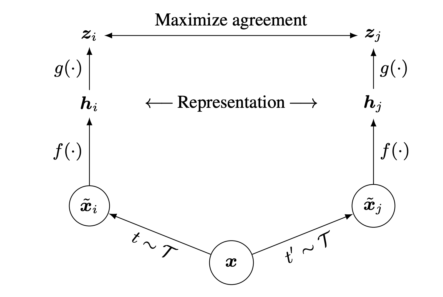 Fig 1. SimCLR: Overview of SimCLR Framework [1].
Encoder
A base encoder extracts features from each augmented view. This encoder learns meaningful visual representations without labels.
Projection Head
The encoder output is passed into a small MLP projection head:
\[z = \text{MLP}(h)\]This projection improves the quality of contrastive learning; the encoder’s representation $h$ is used for downstream tasks.
NT-Xent Contrastive loss
SimCLR uses the NT-Xent (Normalized Temperature-Scaled Cross Entropy) loss to maximize similarity between positive pairs and minimize similarity with negative samples:
\[\ell_{i,j} = - \log \frac{ \exp(\operatorname{sim}(z_i, z_j)/\tau) }{ \sum_{k \neq i} \exp(\operatorname{sim}(z_i, z_k)/\tau) }\]$\tau$ is the temperature parameter controlling distribution sharpness. Appropriate temperature parameter can help model learn from hard negative samples. sim() is cosine similarity. (i, j) is a positive pair, and all other images in the batch act as negatives.
2. Workflow
- Sample a batch of N images.
-
Applying two independently sampled data augmentations to each image. \(x \rightarrow x_i',\, x_j'\) This produces two correlated views of the same image. All other augmented images in the batch serve as negative examples.
-
Each augmented view is passed through the encoder to obtain representations:
\[h = f_{\text{encoder}}(x')\] -
The projection head maps representations into a space where contrastive loss is applied:
\[z = g_{\text{proj}}(h)\] - SimCLR uses the NT-Xent loss to increase similarity between positive pairs and decrease similarity with negative samples.
3. Key Findings
Experiment Setting: Using ResNet-50 as base encoder, and two layer MLP projection head. Training at 4096 batch size and 100 epoches. SimCLR able to achieve 76.5% Top-1 accuracy on ImageNet[1].
Large Batch Sizes: SimCLR demonstrates that more negative samples is better for contrastive learning. However, training large batch using standard SGD/Momentum is unstable. Therefore, SimCLR uses LARS optimizer.
Data Augmentation: SimCLR relies on strong augmentations (crop, color jitter, Gaussian blur, etc.) to create meaningful positive pairs. No single augmentation (e.g., only cropping or only color jitter) is sufficient to learn high-quality representations. The model can still solve the contrastive prediction task with high accuracy, but the representations remain poor unless augmentations are combined, as shown in Fig 2 that the diagnoal entries are lower than off-diagnoal entries. A particularly important finding is that the composition of random cropping + random color distortion produces the strongest results. If only using random cropping, network will find the shortcut that most patches will share similar color distribution[1].
Contrastive learning benefits from bigger model and longer training.
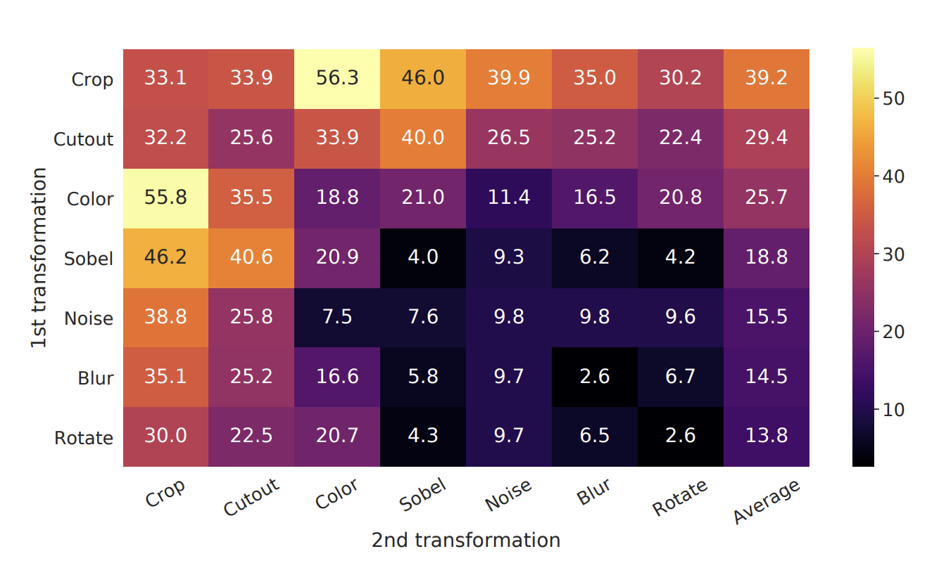 Fig 2. Impact of combining data augmentations on representation quality in SimCLR [1].
Masked Image Modelling (MAE)
Masked Autoencoders are a self-supervised learning method for masked image modeling. The model learns to reconstruct missing image patches using only a set of visible patches[2].
1. Model Structure
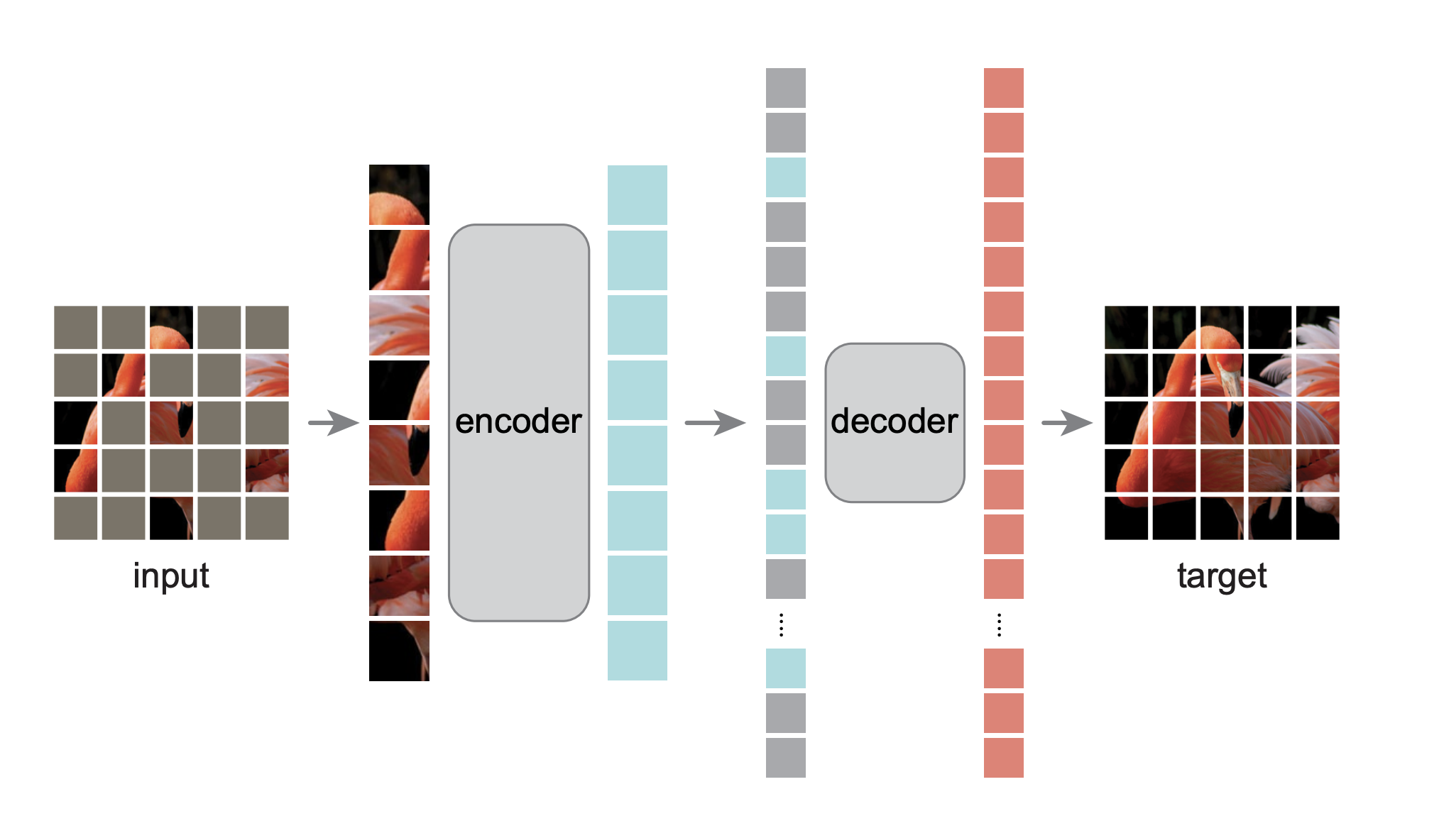 Fig 2. Architecture of Masked Autoencoders (MAE) [2].
Asymmetric Encoder
The encoder is a ViT that only processes visible patches. Because only small part of image is visible to encoder when using high masking ratio, the encoder computation and memory cost are substantially reduced. The encoder learns semantic, high-level features.
Lightweight Decoder
The decoder receives both the encoded visible patch embeddings and a set of mask tokens that represent missing patches. Mask tokens are shared learned vectors with positional embeddings indicates where a patch should appear. The decoder reconstructs pixel values for all patches, and its output channel equals the number of pixels per patch, which is later reshaped back into image format. The decoder is used only during pre-training, not for downstream tasks, hence the design of it can be lightweight.
Normalized Pixel Reconstruction Variant
MAE also evaluates reconstruction using normalized pixel values rather than raw RGB pixel values.
\[\tilde{x} = \frac{x - \mu_{\text{patch}}}{\sigma_{\text{patch}}}\]Using normalized targets prevents the model from overfitting to global color biases and encourages learning of structure, texture, and spatial patterns, which are more useful for downstream tasks.
2. Workflow
The MAE pre-training pipeline works as follow:
- Split input image into non-overlapping patches and convert them into token via linear projection.
- Random shuffle patch tokens and select a subset as visible tokens; rest of patches will be masked.
- Feed only the visible patch tokens into the ViT encoder. The encoder will output latent representations for visible patches.
- Create mask tokens for all removed patches and append mask tokens to encoder outputs.
- Unshuffle the sequence to restore the original spatial ordering.
- Feed the visible embeddings + mask tokens into decoder.
- The decoder predicts pixel values for all patches.
- Compute MSE loss only using masked patches. For Masked patches M,
3. Key Findings and Results
Experiment Setting:
Pre-training performed on ImageNet-1K using ViT-Large (ViT-L/16) as the backbone.
Result: Baseline MAE with ViT-L achieve 84.9% accuracy on ImageNet-1K, while using ViT-H can achieve 87.8% accuracy[2].
Masking Ratio: A very high masking ratio of around 75% works best for both linear probing and fine-tuning, which shows that MAE benefits from massive masking[2]. This is because high masking ratio prevent model from simply learning from surrounding patches without learning from high-level information. In addition, the authors show that an MAE pre-trained with a 75% mask ratio can still produce plausible reconstructions even when evaluated with much higher masking ratios, demonstrating strong generalization of the learned representations.
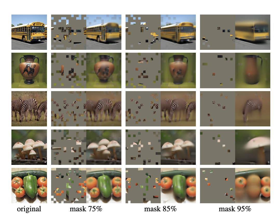 Fig 2. MAE reconstructions under increasing masking ratios [2].
Decoder Depth: A shallow decoder yields weaker linear-probing accuracy because the encoder must learn too many low-level details that should normally be handled by the decoder.
Mask Token Placement: Adding mask tokens after the encoder is better than adding them before. This is because encoder processes only real image data, which improves representation quality and save memory and compute.
Normalized Pixel Targets: Predicting normalized pixel values significantly improves reconstruction quality and downstream performance, as encoder is encouraged to learn structure, shape, and texture, instead of memorizing absolute pixel colors.
Minimal Augmentation: MAE performs well without strong data augmentation. Unlike contrastive learning such as SimCLR, MAE relies primarily on the masking operation as its augmentation.
DINO: self-distillation with no labels
DINO (self-distillation with no labels) is a self-supervised learning framework based on knowledge co-distillation, where a student network is trained to match the output distribution produced by a teacher network[3].
Both networks share the same architecture (e.g., ViT or ResNet) and consist of a backbone encoder followed by a projection head.
Model Structure
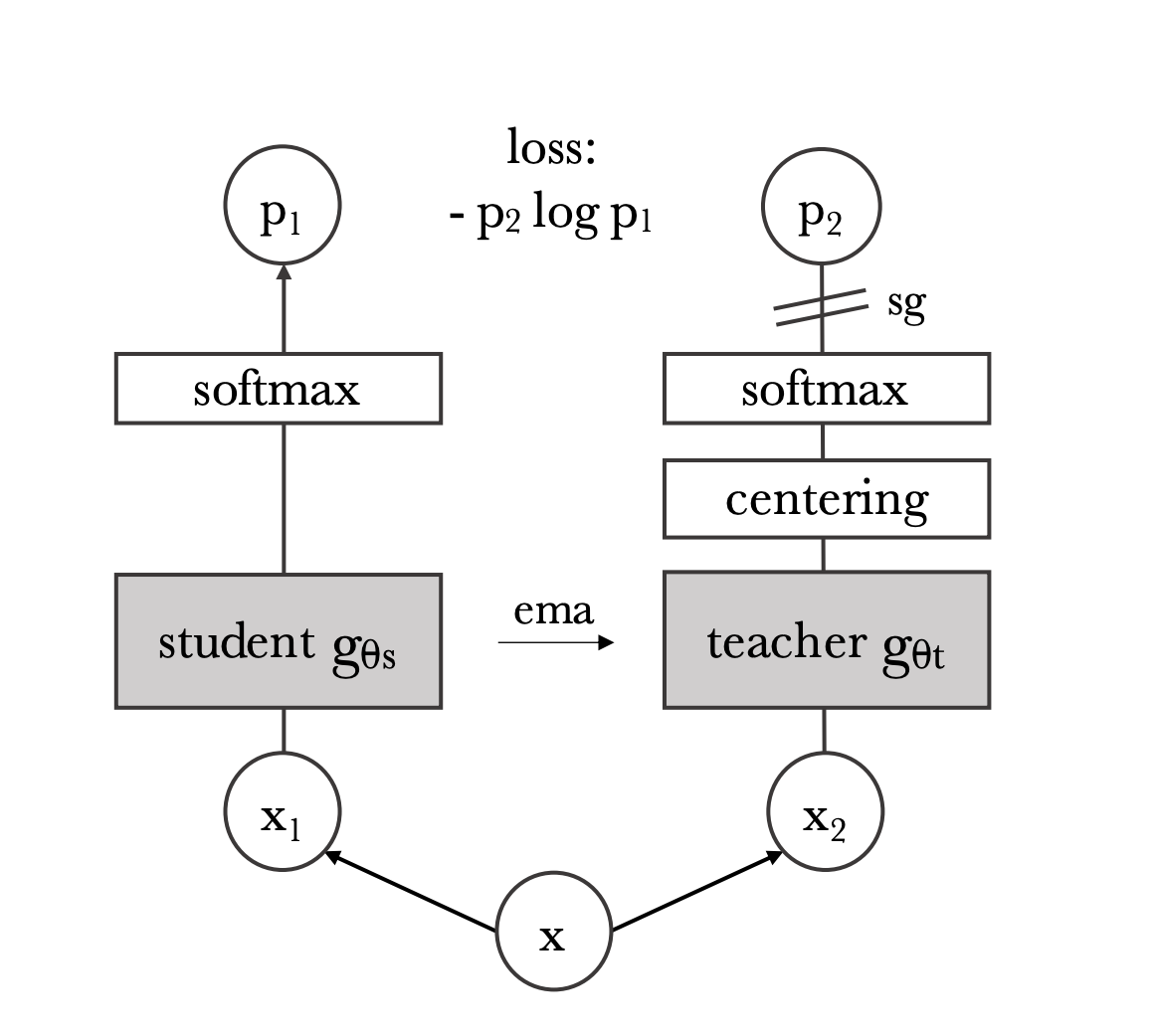 Fig 5. Teacher-Student Training Framework in DINO [3].
Teacher-Student Symmetry
Student and teacher have identical network structures. Only the student receives gradient updates via SGD. The teacher parameters are updated using an exponential moving average (EMA) of the student:
\[\theta_{\text{teacher}} \leftarrow \alpha \theta_{\text{teacher}} + (1-\alpha)\theta_{\text{student}}\]where \(\alpha\) follows a cosine schedule increasing from 0.996 to 1.
Output distribution
Both networks produce a probability distribution by applying a softmax with temperature:
\[P = \text{softmax}\!\left(\frac{z}{\tau}\right)\]The student uses a higher temperature \(\tau\) to avoid over-confidence, while the teacher uses a low temperature \(\tau\) to produce informative targets.
Workflow
-
Given an input image, DINO generates a set of augmented views V: (1) Two global crops x1 and x2 (resolution 224 × 224), (2) multiple local crops (resolution 96 × 96).
-
Teacher only processes global views, and student processes all crops. This asymmetry teaches the student viewpoint invariance and encourages learning high-level semantic representations.
-
The objective is to make the student output distribution match the teacher’s across corresponding views. This is done by minimizing the cross enrtopy loss with respect to student parameter:
\[L = - \sum_{k} P^{(t)}_{k} \log\left(P^{(s)}_{k}\right)\]
where \(P^{(t)}_{k}\) denotes the probability from teacher network to the \(k\)-th output dimension, and \(P^{(s)}_{k}\) denotes the probability from the student network. The summation is taken over all output dimensions \(k\).
-
Student network’s parameters are updated via SGD, and teacher network’s parameter are updated using EMA of student weights (no backpropagation).
-
Both networks use a projection head (similar to SwAV) to produce the representations used for distillation. The backbone embeddings are used later for downstream tasks
Key Findings & techniques
Avoiding Collapse: DINO achieves non-trivial representations without negative samples by combining three stabilizing mechanisms:
- Centering: Maintaining balanced activations across dimensions and preventing the model from collapsing to a single dominant feature or neuron.
- Sharpening: Using low-temperature softmax on teacher outputs to ensure teacher outputs are peaked and non-uniform.
- EMA Teacher Updating: Teacher parameters are updated slowly to provide stable optimization in training.
Multi-crop training: DINO reveals that multi-crop training is highly effective for learning viewpoint invariant representations. By training the student on both global and local views while restricting the teacher to global views only, DINO encourages the model to connect fine-grained local details with global semantic context.
Patch size: The performance will be improved if using smaller patch size, even though more memory will be taken.
Semantic properties: The self attention map of DINO-pretrained ViT align well with object boundary as shown in Fig 6, which mean that self-distillation not only improves downstream performance but also leads to learning more interpretable and spatially meaningful representations.
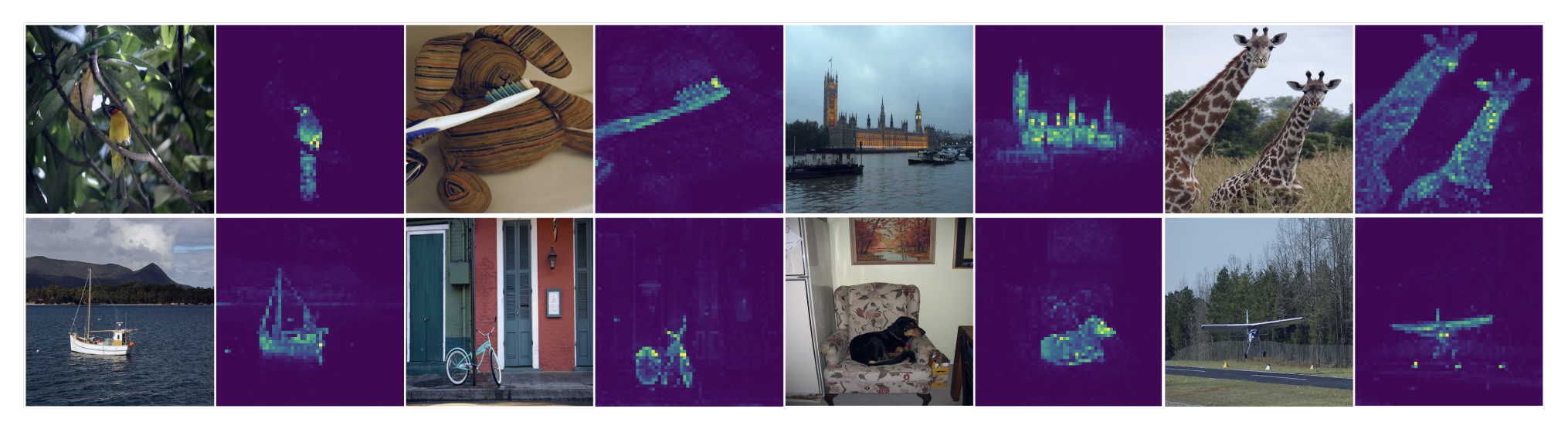 Fig 5. Attention map of DINO pretrained ViT [3].
Conclusion
Self-supervised learning enables models to learn meaningful representations directly from unlabeled data. In this report, we examined three representative self-supervised approaches—SimCLR, Masked Autoencoders (MAE), and DINO. SimCLR uses strong data augmentations and large batches to learn discriminative representations. MAE approaches through the perspective of reconstructing the image, showing that high masking ratios can encourage models to focus on semantic structure rather than low-level pixel statistics. DINO introduces a self-distillation framework without negative samples and uses several stablizing techniques to learn invariant features and prevent collapsing. All these methods utilize the dataset itself to design pretext task and reduce reliance on labeled data while achieving competitive performance. As datasets continue to grow in size and labeling costs remain high, self-supervised learning is likely to play an increasingly important role in modern computer vision systems.
Reference
[1] Chen, T., Kornblith, S., Norouzi, M., & Hinton, G. (2020). A simple framework for contrastive learning of visual representations. In International Conference on Machine Learning (pp. 1597-1607). PMLR.
[2] He, K., Chen, X., Xie, S., Li, Y., Dollár, P., & Girshick, R. (2022). Masked autoencoders are scalable vision learners. In Proceedings of the IEEE/CVF Conference on Computer Vision and Pattern Recognition (pp. 16000-16009).
[3] Caron, M., Touvron, H., Misra, I., Jégou, H., Mairal, J., Bojanowski, P., & Joulin, A. (2021). Emerging properties in self-supervised vision transformers. In Proceedings of the IEEE/CVF International Conference on Computer Vision (pp. 9650-9660).