Exploring Modern Novel View Generation Methods
[Project Tack] Historically, novel view synthesis (NVS) has relied on volumetric radiance field approaches, such as NeRF. While effective, these methods are often computationally expensive to train and prohibitively slow to render for real-time applications. To address these limitations, researchers have developed new architectures that reduce computational costs while maintaining or exceeding visual fidelity. This report examines two distinct solutions to this challenge: 3D Gaussian Splatting (3DGS) and the Large View Synthesis Model (LVSM).
Current Novel View Generation Methodologies
3D Gaussian Splatting
Note: This section provides an overview of 3D Gaussian Splatting based on the original paper by Kerbl et al. [1]. All figures and methodology descriptions are derived from their work.
Overview
Following Radiance Field-based methods such as NeRF, researchers identified a critical bottleneck: achieving high visual quality required computationally expensive training and rendering. While high-fidelity results were possible, they were too slow for real-time applications. Conversely, methods optimized for speed often sacrificed visual detail. Before this paper, real-time, high-resolution rendering (1080p) of unbounded and complete scenes was not achievable without compromising quality. 3D Gaussian Splatting introduced three key elements that maintained state-of-the-art visual quality while enabling competitive training times and real-time novel-view synthesis.
- Represent the scene with 3D Gaussians, which avoids unnecessary computation in empty space in volumetric radiance fields
- Perform interleaved optimization and density control to achieve an accurate representation of the scene
- Develop a fast visibility-aware rendering algorithm that accelerates training and allows real-time rendering
Method
Given input images with known camera intrinsics and extrinsics obtained via Structure-from-Motion (SfM), 3D Gaussian Splatting constructs an explicit radiance field representation using a set of anisotropic 3D Gaussian primitives. The goal of this method is to synthesize a novel target image corresponding with a target camera pose.
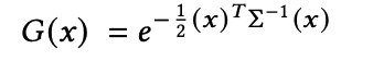
The Gaussians are defined by a full 3D covariance matrix \(\Sigma\) in 3D space, centered at a mean point \(\mu\). The following equation defines how strongly a Gaussian contributes at a given point \(x\), based on the pixel’s distance from the mean.
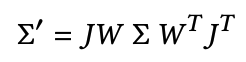
Through the blending process, the Gaussian is multiplied by \(\alpha\). In order to project the 3D Gaussian to a 2D image for rendering, a 2D covariance matrix \(\Sigma'\) must be calculated to define the ellipse shape of the Gaussian splat in image space. \(J\) represents the Jacobian of the affine approximation of the projective transformation, while \(W\) applies the world-to-camera transform to the covariance, effectively handling the rotation of the camera extrinsics for the novel view.
Optimizing the covariance matrix \(\Sigma\) to obtain 3D Gaussians that represent the radiance field is the right idea. However, covariance matrices must be symmetric and positive semi-definite to have meaning in physical space, and gradient updates could easily lead to the matrix becoming invalid. Instead, by defining the matrix using a scaling matrix \(S\) and rotation matrix \(R\), the corresponding \(\Sigma\) can be found. These parameters can be trained in such a way that preserves the positive semi-definite, symmetric nature of \(\Sigma\).
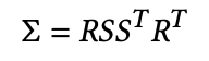
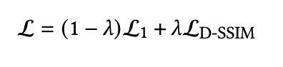
By storing both factors separately, a 3D vector \(\mathbf{s}\) for scaling and a quaternion \(\mathbf{q}\) for rotation, they can be trivially converted to their respective matrices by normalizing \(\mathbf{q}\) to obtain a valid unit quaternion. Stochastic Gradient Descent is used for optimization, with a loss function combining \(L_1\) and a D-SSIM term for photometric loss.
A key aspect of capturing scene complexity with this method is the adaptive control of 3D Gaussians during training so the representation matches the scene by dynamically adding, splitting, and removing 3D Gaussians during training. The previously mentioned \(\alpha\) is used here to control the opacity of Gaussians and effectively measures how much a Gaussian contributes to a rendered image. When Gaussians have persistently low opacity they are pruned, which prevents wasted computation on empty space and is a key reason for the computational efficiency of this approach. On the other hand, large Gaussians are split in this step to allow for a better fit of detailed surfaces, and Gaussians with large gradients are duplicated to increase local density.
Finally, the key aspect of the method that allows for incredibly competitive training times and real-time rendering is the Fast Differentiable Rasterizer for Gaussians. This custom GPU rasterization is designed to efficiently render and differentiate through large numbers of anisotropic Gaussian splats, while avoiding the scalability and gradient-truncation issues of prior splatting methods. It is created with three main objectives: fast rendering and sorting of Gaussian splats, correct (or near-correct) alpha blending for anisotropic Gaussians, and unrestricted gradient flow. The key idea is to sort all Gaussian splats once per image, rather than per pixel, and then reuse this ordering during rasterization utilizing a tile-based pipeline. This key innovation allows for 3D Gaussian Splatting to be practical at scale and speed.
Architecture
As opposed to previous state-of-the-art methods such as NeRF, which utilize neural architectures built around MLPs, 3D Gaussian Splatting is an explicit geometric approach built around learnable primitives and rasterization.
The paper proposes a scene-level, non-neural architecture composed of three tightly coupled modules:
- Explicit 3D Gaussian Scene Representation
- Optimization and Adaptive Density Control
- Fast Differentiable Tile-Based Rasterizer
The expressivity is moved from neural layers into the geometric primitives of 3D Gaussians as discussed above. The main training loop and optimization is shown below.
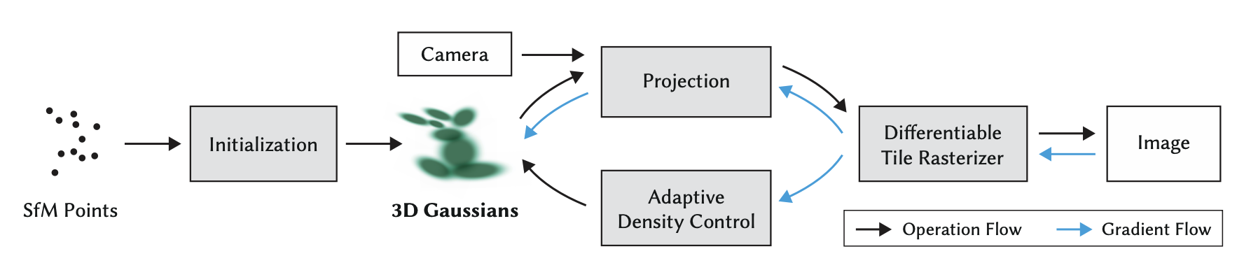
Fig 1. Optimization of sparse SfM point cloud to create a set of 3D Gaussians, which are tiled for the optimization strategy by rasterization [1].
The optimization starts with a sparse SfM point cloud, which is used at initialization to produce the set of initial 3D Gaussian parameters. Each SfM point provides: mean (3D position), isotropic covariance (size), opacity \(\alpha\), and color (via spherical harmonics).
Next, this 3D representation enters the training loop at the projection stage, where camera intrinsics and extrinsics are used as inputs along with the transform of the 3D covariance matrices to create 2D anisotropic covariance matrices. This is effectively the splatting stage of the architecture.
From here, the Differentiable Tile Rasterizer renders the image as described in the methodology above, efficiently creating the 2D pixel-level representation. The rendered image is then compared against the ground-truth training image, and the photometric loss (\(L_1\) + SSIM) is used to compute a gradient that is passed back for SGD.
Passing through the differentiable rasterizer, the gradients flow through both the projection to 3D Gaussians for parameter updates and to the Adaptive Density Control module, which uses these gradients to dynamically adjust the number of Gaussians and the spatial resolution of the representation.
Results
Kerbl et al. tested the model for image synthesis against previous NeRF methods.
The paper evaluated 3D Gaussian Splatting across a diverse set of datasets against 13 real scenes from published datasets and the synthetic Blender dataset. The scenes were chosen for different capture styles, covering both indoor and outdoor environments. Results are compared to state-of-the-art quality methods at the time (Mip-NeRF360) as well as the fastest NeRF methods (InstantNGP and Plenoxels) as benchmarks for quality and speed, respectively.
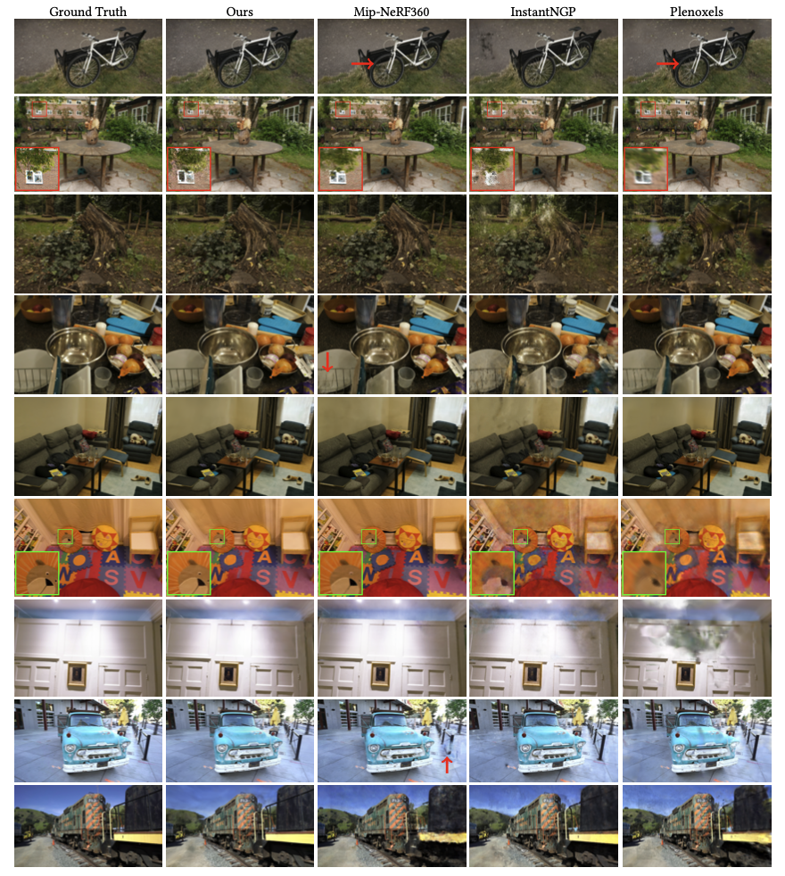
Fig 2. Comparison of 3D Gaussian Splatting to previous methods and ground truth from the Mip-NeRF360 dataset [1].
The image comparisons above demonstrate that 3D Gaussian Splatting achieves comparable quality to Mip-NeRF360. Critical examples are highlighted in each image with zoom-ins or red arrows.
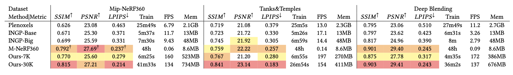
Table 1. Quantitative evaluation of 3DGS (labeled “Ours-7k” and “Ours-30k”) compared to previous work, computed over three datasets. Results marked with a dagger (†) have been directly adopted from the original paper; all others were obtained in the 3DGS paper [1].
For a more quantitative focus, the table above shows that 3D Gaussian Splatting either performs comparably to or outperforms NeRF methods in quality measures, while achieving low training times proportional to quality outputs. A critical value to note is the FPS of 3D Gaussian Splatting, which for the first time enabled real-time rendering speeds. The main drawback, aside from comparison to Plenoxels, is that 3D Gaussian Splatting is highly memory-intensive, requiring significantly more storage than NeRF methods.
Discussion
3D Gaussian Splatting (3DGS) is best understood as a shift in where radiance-field expressivity lives. At the time of the paper, NeRF-style methods were largely state-of-the-art and concentrated representation power inside neural functions, typically through MLPs. 3DGS moves the representational power to a large set of explicit, learnable primitives—anisotropic Gaussians—so that rendering can become closer to typical software rasterization of computer scenes rather than volumetric ray marching, which is much more computationally intensive and less parallelizable. This effectively removes a bottleneck that had prevented previous real-time novel view synthesis at high resolution. By rendering only the primitives that project onto the screen and compositing them efficiently, 3DGS avoids wasting computation on empty space and achieves high framerates without sacrificing radiance-field-style image formation.
3DGS couples this effective representation with an optimization strategy that refines the structure of the image. Beyond strict updates of Gaussian attributes, the method also adaptively changes the representation through pruning and densification of existing Gaussians. This helps improve reconstruction while avoiding wasted computation.
The rasterizer architecture is what makes this approach feasible, as it accelerates both training and inference while preserving differentiability and stable gradient flow. As with most performance-driven designs, the tile-based pipeline trades compute for memory: the same tiling and primitive management that enable speed also increase the storage footprint, making 3DGS substantially more memory-intensive due to the large number of stored primitives.
Overall, 3DGS takes a fundamentally different approach from previous methods of radiance-field-quality novel view synthesis by storing representational power in 3D Gaussian primitives and utilizing optimizations and architecture to make it feasible. This leads to a tradeoff: substantially faster rendering with competitive visual quality, but high memory costs.
Running the Codebase
We use the popular open-source implementation OpenSplat [3], since it includes detailed instructions for building on different OSes as well as on Colab. On MacOS, it was as simple as installing the dependencies with brew, cloning the repository, and running
cmake -DCMAKE_PREFIX_PATH=/path/to/libtorch/ .. && make -j$(nproc).
./opensplat ../data/banana -n 2000 finished running in around 2 minutes and produced the expected banana model, viewed on https://antimatter15.com/splat/.
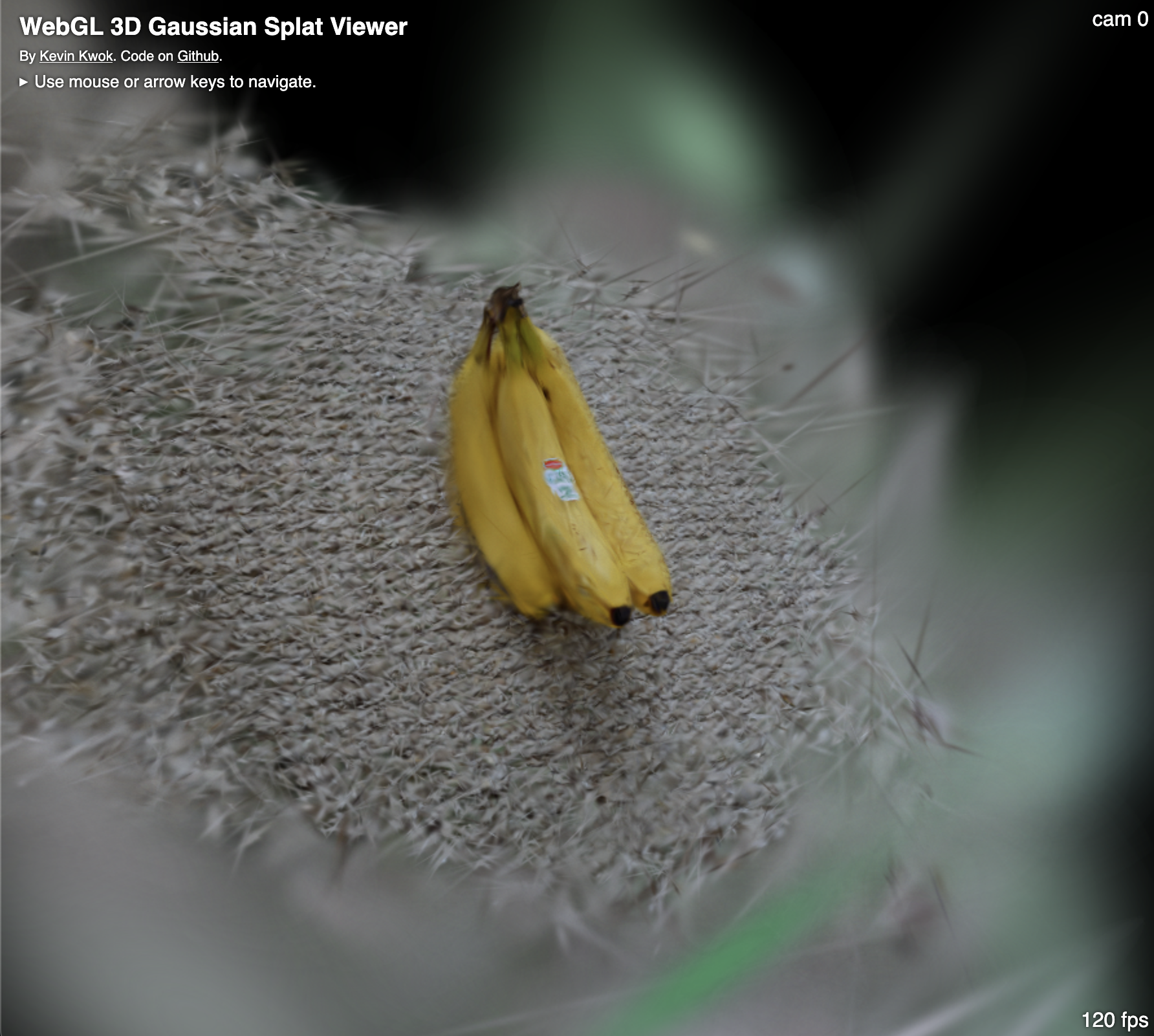
Fig 3. Banana splat rendered on antimatter
Creating a Dataset
To explore the full Gaussian splatting pipeline, we recorded a 1-minute video on an iPhone 14 Pro walking around some objects on a table. Effort was made to minimize motion blur and capture as many reference views of the objects as possible.
The first step afterwards was to extract the frames from the video. ffmpeg worked nicely, with the following producing 173 images:
subprocess.run([
    "ffmpeg",
    "-i", str(video),
    "-vf", "fps=3,scale=iw*0.75:ih*0.75",
    "-q:v", "2", # quality, 0 is highest
    str(out / "%06d.jpg"),
], check=True)
We then ran the extracted frames through a structure-from-motion (COLMAP) pipeline to get it ready for OpenSplat:
# feature extraction
run_command([
    colmap_bin, "feature_extractor",
    "--database_path", database_path,
    "--image_path", input_images_dir,
    "--ImageReader.camera_model", "PINHOLE",
    "--ImageReader.single_camera", "1"
])

# sequential matching
run_command([
    colmap_bin, "sequential_matcher",
    "--database_path", database_path,
    "--SequentialMatching.overlap", "10",
    "--SequentialMatching.loop_detection", "0"
])

run_command([
    colmap_bin, "mapper",
    "--database_path", database_path,
    "--image_path", input_images_dir,
    "--output_path", sparse_path
])

# image undistortion
run_command([
    colmap_bin, "image_undistorter",
    "--image_path", input_images_dir,
    "--input_path", sparse_path / "0",
    "--output_path", output_path,
    "--output_type", "COLMAP",
    "--max_image_size", "2000"
])
Much debugging later, we were able to get a passable reconstruction of our video.
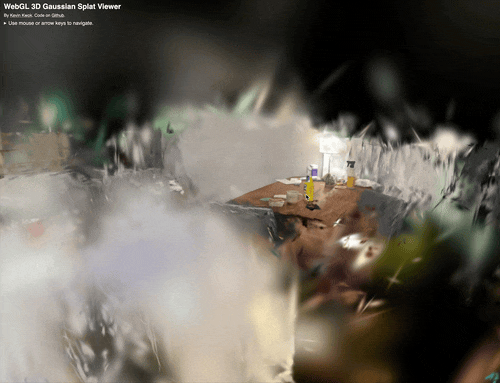
Fig 4. Splat of a team member’s dining table after frame extraction, SfM, and OpenSplat
Exploring Activation Functions
The paper applies a sigmoid activation to per-Gaussian opacity (α) to constrain it in the [0, 1) range and an exponential activation to the covariance scale parameters in the name of smooth gradients. We investigate Softplus as an alternative covariance scale activation choice and evaluate its impact on reconstruction quality.
In Gaussian splatting, the covariance parameters must remain positive to ensure valid Gaussians. The paper enforces this constraint by applying an exponential activation; as a result, the magnitude of the gradient update applied to the scale parameters is directly proportional to the physical size of the Gaussian. This introduces an inductive bias where large Gaussians, typically representing background elements or low-frequency geometry, exhibit high volatility during optimization.
To explore this effect, we replace the exponential activation with the softplus function: Softplus(p) = ln(1+exp(p)). The gradient of this activation with respect to the parameter p is the sigmoid function exp(p) / (1 + exp(p)). As p approaches infinity, the gradient saturates at 1. Unlike the exponential function, Softplus essentially imposes a linear update rule for large Gaussians. Using Softplus activation for covariance scale, we expect to see more stability in large features during optimization.
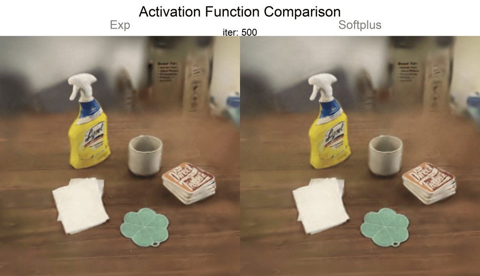 Fig 5. Comparison of Exp and Softplus activation functions over 7000 iterations, view 1
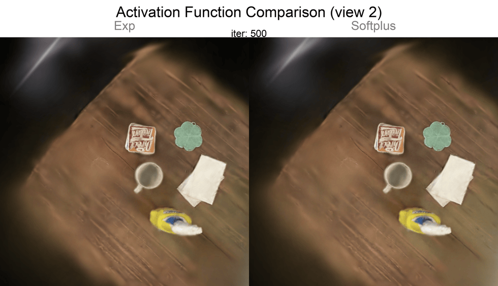 Fig 6. Comparison of Exp and Softplus activation functions over 7000 iterations, view 2
Both models reconstruct the overall scene fairly well, but there are a few noticeable differences. Softplus more accurately one table corner, whereas the exponential activation leaves it somewhat blurry. Softplus also renders the diagonal shadow cast by the rear box more sharply in the first view, aligning more closely with the ground truth images. While not the difference in large Gaussians that we expected, this behavior is still nonetheless interesting.
A possible explanation is related to covariance stability: the exponential activation causes Gaussians to expand and contract aggressively, relying on later density control to correct their scale. Compared with the smoother, more stable behavior of softplus, this dynamic may make it harder for exp to resolve thin structures like table edges or shadows within 7,000 iterations.
These results are thus suggestive rather than definitive. Evaluating on a higher-quality dataset (i.e. not from a self-captured iPhone camera) and running for the recommended 30,000 iterations would help determine whether the observed advantages persist or simply reflect statistical noise.
Large View Synthesis Model (LVSM)
Note: This section provides an overview of the Large View Synthesis Model based on the original paper by Jin et al. [2]. All figures and methodology descriptions are derived from their work.
Overview
Despite advances such as 3D Gaussian Splatting and many variants, existing models prior to the Large View Synthesis Model (LVSM) are encoded with 3D inductive bias (assumptions that are built in about how the 3D world is structured). For example, assumptions that use triangle meshes, NeRF volumetric fields, and 3D Gaussians all encode biases about how the world is a 3D scene and images are projections of that scene. While 3D inductive bias is important to making learning feasible, it can be seen as a bottleneck for data-driven 3D understanding, which led to researchers \(\textbf{aiming to minimize 3D inductive biases}\) with a data-driven approach using LVSM [2]. Additionally, these prior models are trained per scene while the decoder-only LVSM is able to perform zero shot generalization, allowing it to quickly generate novel views of a specific scene without pre-training.
Method
Given \(N\) sparse input images with known camera poses and intrinsics, LVSM synthesizes a target image \(I_t\) under novel target camera extrinsics and intrinsics. For each input view, pixel-wise Plücker ray embeddings \(P_i \in \mathbb{R}^{H \times W \times 6}\) are computed from the camera parameters and patchified together with the corresponding RGB images. Each image–ray patch is concatenated and projected into a latent token via
\[x_{ij} = \mathrm{Linear}_{\text{input}}([I_{ij}, P_{ij}]) \in \mathbb{R}^d,\]forming a sequence of geometry-aware input tokens.
The target camera is represented analogously by computing its Plücker ray embeddings which are then patchified and mapped into patch-wise query tokens
\[q_j = \mathrm{Linear}_{\text{target}}(P^t_j) \in \mathbb{R}^d.\]A transformer model \(M\) conditions the target query tokens on the full set of input tokens to synthesize the novel view:
\[y_1, \ldots, y_{\ell_q} = M(q_1, \ldots, q_{\ell_q} \mid x_1, \ldots, x_{\ell_x}),\]where each output token \(y_j\) encodes the appearance of the \(j\)-th target patch. The output tokens are decoded into RGB patches using a linear projection followed by a sigmoid activation,
\[\widehat{I}^t_j = \mathrm{Sigmoid}(\mathrm{Linear}_{\text{out}}(y_j)),\]and the predicted patches are reshaped and assembled to form the synthesized novel view \(\widehat{I}_t\).
\(\textbf{Loss}\): The model is trained end-to-end using photometric novel view rendering losses:
\[L = \mathrm{MSE}(\widehat{I}^t, I^t) + \lambda \cdot \mathrm{Perceptual}(\widehat{I}^t, I^t),\]where \(\lambda\) balances the pixel-wise and perceptual reconstruction terms.
Architecture
The paper introduces the Large View Synthesis Model (LVSM), “a novel transformer-based framework that synthesizes novel-view images from posed sparse-view inputs without predefined rendering equations or 3D structures…”. The paper also introduces two new architectures using this framework.
The first is an \(\textbf{encoder-decoder LVSM}\). It consists of an encoder, which takes in image tokens and encodes them into a fixed number of 1D latent tokens. This functions as the learned scene representation, which is used to decode novel-view images from. The second is a \(\textbf{decoder-only LVSM}\), which directly takes images and creates novel-view outputs. There is no scene representation in this model. The model’s learning of a direct mapping makes it more scalable, and can use many images to inform the mapping learned. Both, with no assumptions about the 3D world and how it is rendered, are solely data-based and achieve superior quality to existing models, even with reduced computational resources.
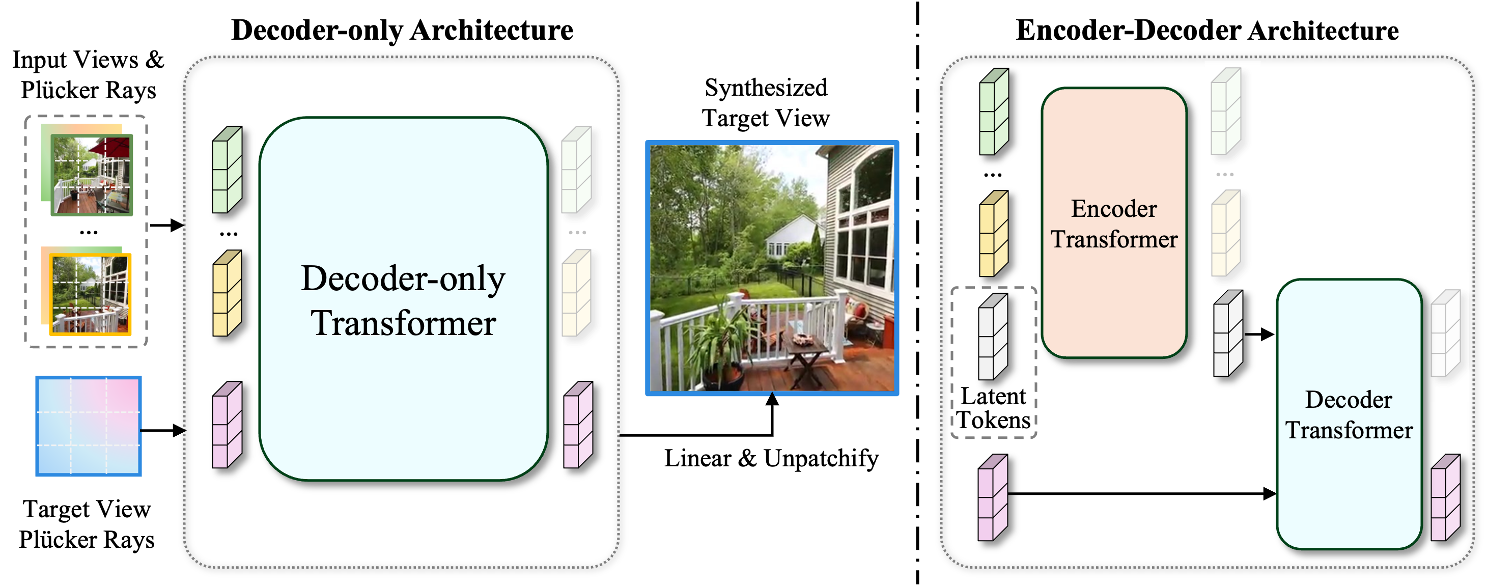
Fig 7. LVSM architectures: (a) Encoder-Decoder LVSM and (b) Decoder-Only LVSM [2].
Results
Jin et al. evaluated LVSM across multiple datasets against previous state-of-the-art methods for both object-level and scene-level novel view synthesis. Here are the quantitative results:
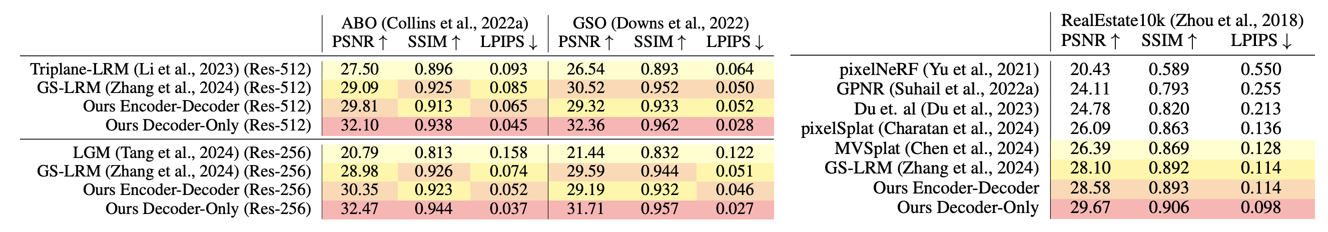
Table 2. Quantitative comparisons on object-level (left) and scene-level (right) view synthesis. Table taken from LVSM paper [2].
For object level testing, they used the Objaverse dataset to train the LVSM. Then, they tested on two object-level datasets, Google Scanned Objects (GSO) and Amazon Berkeley Objects (ABO). Based on the results, the 512-res decoder achieves a 3 dB and 2.8 dB PSNR (Peak Signal-to-Noise Ratio) against the best prior method GS-LRM (which uses 3D Gaussian splatting) and the 256-res decoder only LVSM performs a lot better than Large Multi-view Gaussian Models and GS-LRM. The results show that removing the 3D inductive bias is effective. A strong performance on the ABO dataset also suggests that the model can handle challenging materials difficult for current handcrafted 3D representations.
For scene level testing, they compared the results of LVSM with pixelNeRF, GPNR, pixelSplat, MVSplat, and GS-LRM. The LVSM shows a 1.6 dB PSNR gain against the best prior work GS-LRM, and the improved performance can be visualized in the below image where the LVSM has better performance on thin structures and specular materials.
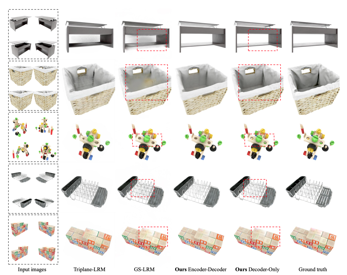
Fig 8. Qualitative comparison for object level testing [2].
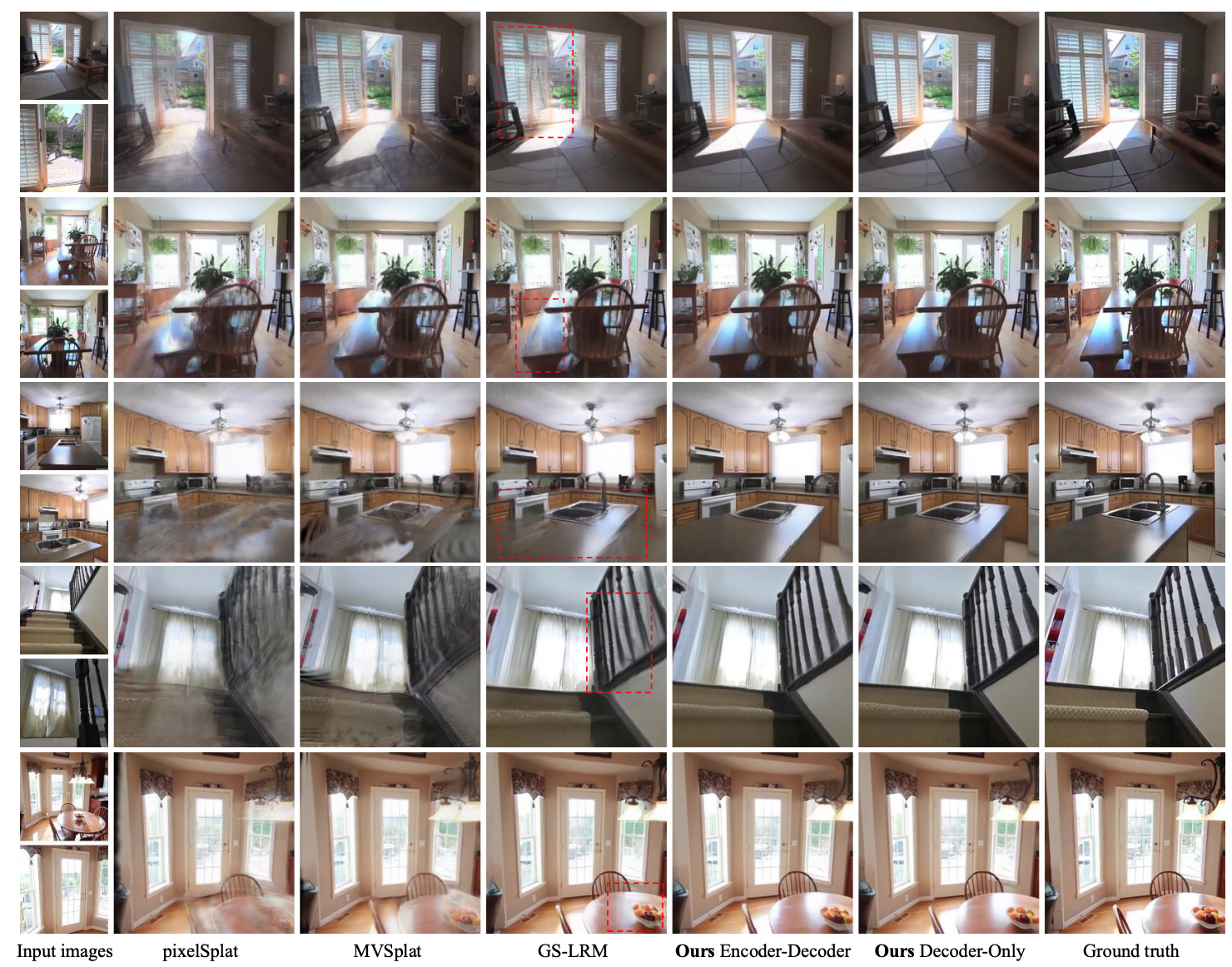
Fig 9. Qualitative comparison on the RealEstate10K dataset for scene level testing [2].
Discussion
The decoder-only model shows better performance with more input views, which shows the model is scalable at test time. On the other hand, the encoder-decoder model shows a performance drop with more input views, suggesting the intermediate representation inhibits performance when trying to compress input information. With only one input, however, the performance is competitive. The improvement in performance validates this data-driven approach, with the goal of minimizing 3D inductive bias.
The decoder-only model, while able to work with many images and can scale well, falls short due to the same property that makes it notable. The direct mapping from input image to novel view means linear increase in image tokens and quadratic growth in complexity. The encoder-decoder model, on the other hand, shows consistent rendering speed as there is always a fixed length set of 1D latent tokens, regardless of the number of input images.
Overall, the LVSM bypasses 3D representations, minimizing 3D inductive bias by using a data-driven approach, and demonstrates an improvement in performance across a variety of benchmarks.
Running the Codebase
Using the paper’s Github repository, we tried running the LVSM ourselves within Google Colab, modifying the code to suit the Colab environment. However, we ran into a few issues with Colab package installation, outdated NumPy code, and related dependency conflicts. In the end, we ran the inference step on 30 inputted images, but the output rendered view consisting of the synthesized views turned out to be a lot blurrier than expected. Some possibilities include sparse inputs, incorrect COLMAP generated images, and low resolution outputs.
Here is the rendered video output for a scene containing a long desk at the library. As you can see, the video shows blurriness as it transitions from one input image to the next input image while attempting to synthesize novel views. Video Link
To view the Colab notebook we used, please refer to this link.
Conclusion
The exploration of 3D Gaussian Splatting and the Large View Synthesis Model shows a variety of approaches in novel-view synthesis, from geometry-based approaches to data-driven paradigms. 3D Gaussian Splatting demonstrates that explicit representations using Gaussians can achieve real-time performance and photorealistic quality through efficient rendering and adaptive optimization but at a high memory cost. LVSM challenges the need for strong 3D inductive biases, achieving competitive results by leveraging transformer architectures and large-scale training for generalizable view synthesis. Together, these approaches illustrate two distinct paths toward faster, more flexible, and increasingly general 3D scene understanding.
Reference
[1] Kerbl, Bernhard, et al. “3D Gaussian Splatting for Real-Time Radiance Field Rendering.” ACM Transactions on Graphics (SIGGRAPH), vol. 42, no. 4, 2023.
[2] Jin, Haian, et al. “LVSM: A Large View Synthesis Model with Minimal 3D Inductive Bias.” arXiv.org, 2 Apr. 2025, arxiv.org/abs/2410.17242.
[3] Pierotofy. “Pierotofy/OpenSplat: Production-Grade 3d Gaussian Splatting with CPU/GPU Support for Windows, Mac and Linux 🚀.” GitHub, 2024, github.com/pierotofy/OpenSplat.