Novel View Synthesis
In computer graphics and vision, novel view synthesis is the task of generating images of a scene given a set of images of the same scene taken from different perspectives. In this report, we introduce three important papers attempting to solve this task.
- 3D Gaussian Splatting
- LVSM: A Large View Synthesis Model With Minimal 3D Inductive Bias
- RayZer: A Self-supervised Large View Synthesis Model
- References
3D Gaussian Splatting
Before 3D Gaussian Splatting (3DGS) [6] was introduced, the dominant paradigm in novel view synthesis was Neural Radiance Fields (NeRF) [5]. NeRF showed strong performance, but its training optimization and rendering were slow. 3DGS introduced a new, explicit scene representation that is fast enough to support rendering in real time.
Method
Differentiable 3D Gaussian Splatting
Previous neural point-based methods, such as [9], computed the color \(C\) of a pixel by blending the colors of the points in the scene representation overlapping the pixel through the equation
Here, \(c_i\) is the color of a point and \(\alpha_i\) is its rendering opacity. This is similar to the formulation used in Neural Radiance Fields. Notably, the point-based approach is discrete and doesn’t require the expensive random sampling approach to calculate color that NeRF requires. 3DGS uses the same rendering equation as [9], but does not rely on neural networks, which are expensive to query, and it models the scene with anisotropic 3D Gaussians instead of points. Each 3D Gaussian is defined by a full 3D covariance matrix in the world coordinate system
They also have their own associated opacity \(\alpha\), which they are multiplied by during rendering.
The 3D Gaussians need to be projected to 2D for rendering, and the covariance matrices after this projection must be calculated. However, due to the fact that covariance matrices need to be positive semi-definite to have physical meaning, they are not optimized directly. Instead, the scaling matrix \(S\) and rotation matrix \(R\) for each Gaussian, which may be converted into the covariance matrix through the equation
are optimized. The scaling is stored in a 3D vector \(s\) and the rotation is stored in a quaternion \(q\) during optimization.
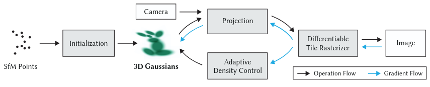 Fig 1. The 3D Gaussian Splatting Framework. The 3D Gaussians are initialized with SfM and repeatedly updated by rendering the training views, comparing them to the ground truth, and applying Stochastic Gradient Descent.
Optimization with Adaptive Density Control of 3D Gaussians
In addition to the position \(p\), opacity \(\alpha\) and covariance \(\Sigma\) of each 3D Gaussian, Spherical Harmonic (SH) coefficients that capture the view-dependent color of each Gaussian are optimized. During the optimization algorithm, the 3D Gaussians are rendered with alpha-blending at each iteration. They are then compared to the training views, and the parameters of the scene are updated through backpropagation with Stochastic Gradient Descent. The sparse pointcloud from SfM is used to initialize the centers of the Gaussians. Gaussians with opacity below a certain threshold that are essentially transparent are removed every 100 iterations. Additionally, to allow the amount of scene covered by the Gaussians to expand, a densify operation is performed every 100 iterations. This involves two strategies. First, small Gaussians in regions not adequately covered are cloned to expand the scene geometry covered. Secondly, in regions with Gaussians that are too large to represent its high variance, the large Gaussians are split into smaller Gaussians. To handle “floaters”, which are Gaussians close to the camera that do not correspond to scene geometry, the opacity of the Gaussians is set close to \(0\) every 3000 iterations. The optimization then increases the opacity of Gaussians where necessary, but keeps the opacity of the floaters low. The operation that deletes with low opacity every 100 iterations then removes them.
Fast Differentiable Rasterization
To allow fast rendering of the 3D Gaussians, a custom tile-based renderer is used. The screen is first divided into 16x16 tiles. Gaussians outside of the view frustum or at extreme positions are removed. Since Gaussians may overlap with multiple tiles, an instance of each Gaussian is created for every tile it touches. Each instance is then assigned a key, which combines its depth in the view space with its tile ID. The instances are then sorted with a single GPU Radix sort by their depth. A list of the Gaussians for each tile is generated. During rasterization, a thread block is launched for each tile. For every pixel in the tile, the block traverses the list, accumulating the color and \(\alpha\) values and stopping once a sufficiently high cumulative opacity has been reached.
Results
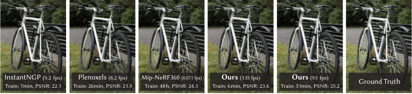 Fig 2. 3D Gaussian Splatting greatly outperforms previous work in terms of training optimization and rendering speed.
The rendering quality of 3D Gaussian Splatting is comparable to those of work before it. However, its training time is much faster. The paper notes that Mip-NeRF360 [10], at the time a state of the art method, took on average 48 hours to optimize a scene and rendered at 0.1 FPS during evaluation, while 3DGS took on average 35-45 minutes, and rendered at over 130 FPS.
Discussion
3D Gaussian Splatting is a landmark paper in novel view synthesis. While it represented a significant step forward from NeRF because of its real-time rendering, its explicit representation has also been useful for future work, which has associated attributes beyond those used for rendering, such as semantic information [11] and motion [12], with the Gaussians.
LVSM: A Large View Synthesis Model With Minimal 3D Inductive Bias
Most existing novel view synthesis methods rely on explicit 3D scene representations, such as NeRF-style volumetric fields [5] or 3D Gaussian Splatting [6]. While effective, these approaches impose strong geometric inductive biases through predefined 3D structures and handcrafted rendering equations. LVSM proposes a fundamentally different approach by minimizing 3D inductive bias and reformulating novel view synthesis as a direct image-to-image prediction task conditioned on camera poses.
Method
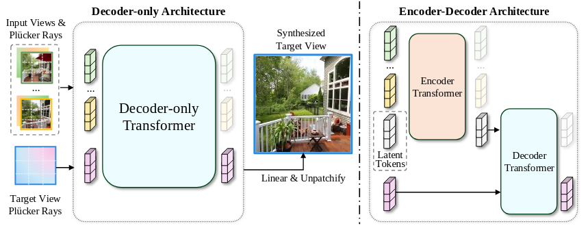 Fig 3. The LVSM Decoder-only and Encoder-Decoder architectures.
Token-Based Representation
Instead of constructing an explicit 3D representation as in NeRF or 3DGS, LVSM operates entirely in token space using a large transformer model. Given \(N\) input images with poses \(\{(I_i, E_i, K_i)\}_{i=1}^N\), LVSM computes pixel-wise Plücker ray embeddings \(P_i \in \mathbb{R}^{H \times W \times 6}\) that encode ray origin and direction in a continuous 6D parametrization. The images and Plücker embeddings are patchified and projected into tokens:
Target views are similarly represented by tokenized Plücker ray embeddings \(q_j\).
Encoder-Decoder Architecture
The encoder–decoder architecture introduces fixed-size learnable latent scene tokens (\(L = 3072\)) that aggregate information from all input views through bidirectional self-attention:
This compact representation enables inference time independent of the number of input views.
Decoder-Only Architecture
The decoder-only architecture processes input and target tokens jointly in a single stream, removing the latent bottleneck:
Although computationally costlier due to quadratic attention, it demonstrates superior scalability with increasing input views.
Both architectures regress RGB values using \(\hat{I}^t_j = \text{Sigmoid}(\text{Linear}_{\text{out}}(y_j))\) and are trained end-to-end with MSE and perceptual loss, without depth supervision or geometric constraints. QK-Normalization stabilizes training.
Results
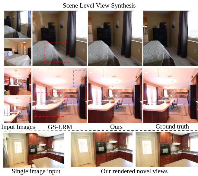 Fig 4. A qualitative comparison between LVSM and GS-LRM on single and multi-view image input.
LVSM achieves state-of-the-art performance on object-level (ABO, GSO) and scene-level (RealEstate10K) datasets, improving PSNR by 1.5–3.5 dB over GS-LRM [2], particularly excelling on specular materials, thin structures, and fine textures. The decoder-only model shows strong zero-shot generalization: trained with four views, it continues improving up to sixteen views. Conversely, the encoder-decoder model plateaus beyond eight views due to its fixed latent representation. Notably, even small LVSM models trained on limited resources outperform prior methods.
Discussion
LVSM demonstrates that high-quality novel view synthesis can be achieved through purely data-driven learning without explicit 3D representations. However, as a deterministic model, it struggles to hallucinate unseen regions, producing noisy artifacts rather than smooth extrapolation. The decoder-only architecture also becomes expensive with many input views.
The superior performance of decoder-only over encoder-decoder reveals an important insight: 3D scenes may resist compression into fixed-length representations. Unlike language, visual information from multiple viewpoints contains redundant spatial structure that degrades when forced through a latent bottleneck, explaining why encoder-decoder performance drops beyond eight views while decoder-only continues scaling.
Overall, LVSM demonstrates that learned representations without structural constraints offer a promising direction for novel view synthesis, echoing the shift from encoder–decoder to decoder-only architectures in large language models.
RayZer: A Self-supervised Large View Synthesis Model
The dominant paradigm in studies on novel view synthesis has been to train models on datasets with COLMAP [3] annotations. However, there are several notable drawbacks to this approach. COLMAP is slow, struggles in sparse-view and dynamic scenarios and may produce noisy annotations. RayZer introduces a groundbreaking new approach to novel view synthesis that is entirely self-supervised (e.g. it does not use any camera pose annotations during training or testing) and thus avoids COLMAP entirely.
Along with SRT [4] and LVSM [1], RayZer falls into the group of novel view synthesis methods employing a purely learned latent scene representation and a neural network to render it. This is in contrast to most state-of-the-art methods, which primarily rely on NeRF [5] or 3D Gaussian [6] representations. These two techniques carry a strong inductive bias through their use of volumetric rendering.
Method
Self-Supervised Learning
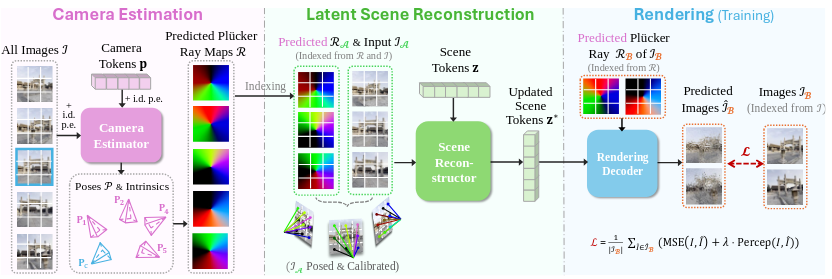 Fig 5. RayZer first predicts camera parameters, then generates a latent scene representation and finally renders novel views.
RayZer is a self-supervised method that takes in a set of unposed, multiview images and outputs camera poses and camera intrinsics, as well as the latent scene representation. The input images are split into two subsets, \(I_A\) and \(I_B\). \(I_A\) is used to predict the scene representation, and \(I_B\) supervises this prediction by producing a loss between the predicted renders of the scene representation corresponding to the predicted camera poses of \(I_B\) and the ground truth.
Camera Estimation
RayZer first patchifies the image and converts the patches into tokens with a linear layer. Both intra-frame spatial positional encodings and inter-frame image index positional encodings are employed. To predict the pose of each camera (with respect to a chosen canonical view), RayZer allows information to flow from the image tokens to camera tokens, with one camera token for each image, by integrating both of them into a transformer, and then decodes them with an MLP. Specifically, the camera tokens are initialized with a learnable value in \(\mathbb{R}^{1 \times d}\). An image index positional encoding is added to them to inform the model which image each camera token corresponds to. The camera estimator consists of several full self-attention layers. Each layer can be written like so:
The first equation describes how the state \(y\) is initialized as the concatenation of \(f\), the initial image tokens, and \(p\), the initial camera tokens. The second equation describes how \(y\) is repeatedly updated by passing it through a self-attention transformer layer. The third equation describes how \(f^{*}\) and \(p^{*}\) are extracted from the final \(y\) value, \(y^{l_T}\).
Finally, the relative pose for each image is estimated with a MLP like so:
where \(p_i\) is the camera token for image \(I_i\) and \(p_c\) is the camera token for the canonical view. The output is parametrized with a continuous 6D representation. Another similar MLP is used to estimate the focal length from the camera token for the canonical view.
Scene Reconstructor
We can generate a Plücker ray map [7] for each image in \(A\) by combining the predicted SE(3) pose \(P_i\) and intrinsic matrix \(K\) (which is derived from the predicted focal length) associated with it. The Plücker ray maps are patchified and then combined with the image tokens of \(A\) along the feature dimension using an MLP. The result of this fusing process is \(x_A\).
In the scene reconstructor, learnable tokens representing the scene reconstruction, \(z \in \mathbb{R}^{L \times d}\), are updated through several transformer layers along with \(x_A\). This mechanism is identical to the one used in the camera estimation module and can be expressed as
\(z^{*}\) is the latent scene representation. \(x_A\) is discarded at the end of the sequence.
Rendering Decoder
The goal of the rendering decoder is to render the scene from novel viewpoints using the latent scene representation. The architecture is inspired by LVSM. To render a target camera, we represent the target camera as a Plücker ray map, tokenize it and use the rule
where \(r^{*}\) are the tokens that are used for rendering and \(r\) is their initial value. \(D_{\text{render}}\) uses the same Transformer layer mechanism as the camera estimation and scene reconstructor modules. Finally, to produce the final RGB image, we decode the render tokens with an MLP like so:
Results
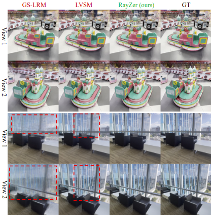 Fig 6. A qualitative comparison between GS-LRM, LVSM and RayZer.
Despite not using any ground truth camera annotations during training or testing, RayZer achieves state of the art performance. It achieves a 2.82% better PSNR, 4.70% better SSIM and 13.6% better LPIPS on the DL3DV-10K dataset [8] compared to LVSM, a leading method in novel view synthesis. The paper highlights how this may be in part due to the noisy nature of COLMAP pose annotations; by avoiding using camera pose data as input, which may be inaccurate, RayZer may have a higher ceiling than methods that rely on them.
Discussion
Perhaps the most compelling and fascinating part about RayZer is that it is able to estimate camera poses without ever being shown ground truth camera pose data. Neural networks tend to work with high-dimensional, abstract features, and it is uncommon to see them estimate simple, understandable values without supervision. This result shows that self-supervised methods have applications to 3D computer vision beyond being used as pre-training strategy
References
[1] Jin, Haian, et al. “LVSM: A Large View Synthesis Model with Minimal 3D Inductive Bias.” arXiv preprint arXiv:2410.17242 (2024).
[2] Zhang, Kai, et al. “GS-LRM: Large Reconstruction Model for 3D Gaussian Splatting.” arXiv preprint arXiv:2404.19702 (2024).
[3] Schonberger, Johannes L., and Jan-Michael Frahm. “Structure-from-motion revisited.” Proceedings of the IEEE conference on computer vision and pattern recognition. 2016.
[4] Sajjadi, Mehdi SM, et al. “Scene representation transformer: Geometry-free novel view synthesis through set-latent scene representations.” Proceedings of the IEEE/CVF Conference on Computer Vision and Pattern Recognition. 2022.
[5] Mildenhall, Ben, et al. “Nerf: Representing scenes as neural radiance fields for view synthesis.” Communications of the ACM 65.1 (2021): 99-106.
[6] Kerbl, Bernhard, et al. “3D Gaussian splatting for real-time radiance field rendering.” ACM Trans. Graph. 42.4 (2023): 139-1.
[7] Zhang, Jason Y., et al. “Cameras as rays: Pose estimation via ray diffusion.” arXiv preprint arXiv:2402.14817 (2024).
[8] Ling, Lu, et al. “Dl3dv-10k: A large-scale scene dataset for deep learning-based 3d vision.” Proceedings of the IEEE/CVF Conference on Computer Vision and Pattern Recognition. 2024.
[9] Kopanas, Georgios, et al. “Neural point catacaustics for novel-view synthesis of reflections.” ACM Transactions on Graphics (TOG) 41.6 (2022): 1-15.
[10] Barron, Jonathan T., et al. “Mip-nerf 360: Unbounded anti-aliased neural radiance fields.” Proceedings of the IEEE/CVF conference on computer vision and pattern recognition. 2022.
[11] Zhou, Shijie, et al. “Feature 3dgs: Supercharging 3d gaussian splatting to enable distilled feature fields.” Proceedings of the IEEE/CVF Conference on Computer Vision and Pattern Recognition. 2024.
[12] Lin, Chenguo, et al. “MoVieS: Motion-aware 4D dynamic view synthesis in one second.” arXiv preprint arXiv:2507.10065 (2025).