Deep Learning for Image Super-Resolution
Image super-resolution is a natural, ill-posed computer vision problem, being the task of recovering a high-resolution, clean image from a low-resolution, degraded image. In this post, we survey 3 recent methods of image super-resolution, each highly distinct with its own advantages and disadvantages. Finally, we conduct an experiment in modifying the structure of one of these methods.
- Background and Introduction
- A Survey of Deep Learning for Super Resolution
- Experiments: An Extension of the Hybrid Attention Transformer
- Conclusion
- References
Background and Introduction
Super-resolution is a natural problem for image-to-image methods in computer vision, referring to the process of using a degraded, downsampled image to recover the original image before degradation and downsampling. Of course, this is an ill-posed problem; two different high-resolution images can downsample and degrade into the same low-resolution image (that is, the process is not injective), so truly inverting the process is impossible. For this reason, we settle for the task of estimating a function that approximates an inverse, producing a high-resolution image based solely on some mathematical assumptions and the information of the low-resolution image. This includes simple, classical methods, such as nearest-neighbor or bicubic upsampling, as well as, in recent years, statistical methods making use of deep learning for computer vision.
We will be surveying three of these recent methods, highlighting the very different ways that one can go about achieving the same end goal in super-resolution:
-
The Hybrid Attention Transformer (HAT), a shifted-window Transformer-based method
-
Look-Up Table (LUT) methods, which use a precomputed table of pixel estimates
-
Unfolding networks, which combine classical model-based methods with learning-based methods
Additionally, we will be discussing an experiment that we carried out involving a modification to the HAT architecture.
A Survey of Deep Learning for Super Resolution
Hybrid Attention Transformer (HAT)
Transformer-based models have recently seen great success for vision tasks, with modifications such as the Swin Transformer further improving these models by reducing computational burdens and reintroducing inductive biases. However, in practice, Swin-based methods often suffer from a small practical receptive field, where the reconstruction prediction of any given pixel is based only upon a small number of pixels near it, even if, in theory, the tokens for that part of the image should have implicitly “seen” all other tokens during self-attention. For this, the Hybrid Attention Transformer (HAT) is designed specifically to utilize a larger portion of the image during reconstruction by combining windowed-self-attention, channel attention, and a novel overlapping-window attention mechanism.
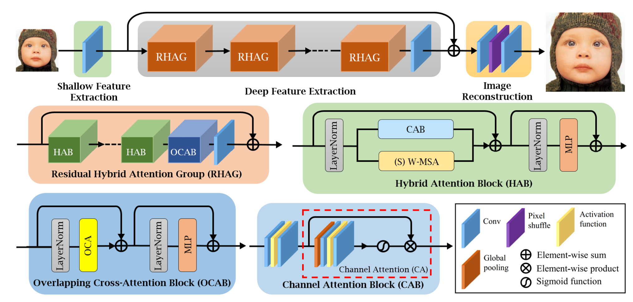
Fig 1. HAT Architecture Overview [1].
Hybrid Attention Block (HAB)
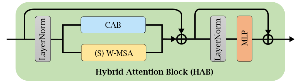
Fig 2. Hybrid Attention Block [1].
The Hybrid Attention Block (HAB) aims to combine the deep flexibility of Vision Transformers with the efficiency and global accessibility of channel attention.
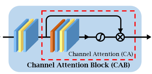
Fig 3. Channel Attention Block [1].
The Channel Attention Block (CAB) consists of two convolutional layers separated by a GELU activation, followed by a channel attention (CA) module. The CA module consists of global average pooling (GAP), followed by two \(1 \times 1\) convolutions, ensuring that the channel number is the same as prior to the CA module, separated by another GELU. Then, the sigmoid function is applied to the now-\(1 \times 1 \times C\)-shaped output to create channel weights, which are multiplied channel-wise by the pre-CA module input, to get an output of the same \(H \times W \times C\) shape, where each channel has been scaled by a factor in \([0, 1]\). The factors are applied globally to each channel and are determined by GAP + convolutions, allowing all channels to utilize information from, to some degree, all positions in all other channels in an efficient manner.
In the HAB, the CAB is inserted into a standard Swin Transformer block after the first LayerNorm in parallel with the window-based multi-head self-attention (W-MSA) module, where they are then combined additively (along with a residual connection). The efficiency and simplicity of the CAB comes at the cost of specific positional information being unutilized due to GAP, which is why the CAB is used in parallel with W-MSA, which explicitly does account for positional information. So, then, for a given input feature \(X\), the HAB is computed as:
\[X_N = \mathrm{LN}(X),\] \[X_M = (\text{S})\text{W-MSA}(X_N) + \alpha\,\mathrm{CAB}(X_N) + X\] \[Y = \mathrm{MLP}(\mathrm{LN}(X_M)) + X_M,\]where LN is the LayerNorm, (S)W-MSA is the (shifted) window-multihead self attention, MLP is the standard positionwise feed-forward network of a Transformer, \(X_N\) and \(X_M\) denote intermediate features, \(Y\) is the output, and \(\alpha\) is a small hyperparameter that tempers the influence of the CAB compared to the W-MSA, to avoid issues of conflict between the two modules during optimization; empirically, \(\alpha=0.01\) was found to give the best performance, as this parallel scheme can introduce significant stability issues in the optimization process if the influence of each branch is not controlled. Within-window linear mappings are used to get \(Q\), \(K\), and \(V\) matrices, though, notably, these mappings are applied on the individual spatial pixels of the input, not on patches (that is, patches of size \(1 \times 1\) are used), as the spatial dimensions of the input need to be maintained throughout the network to account for residual connections. A fixed window size is employed, the same as in the regular Swin Transformer, however, notably, the model does not contain any patch merging, again in service of retaining the shape of the image for residual connections. Within-window attention uses the standard attention scheme, with a fixed sinusoidal relative positional encoding within each window similar to that of “Attention is All You Need”.
Overlapping Cross-Attention Block (OCAB)
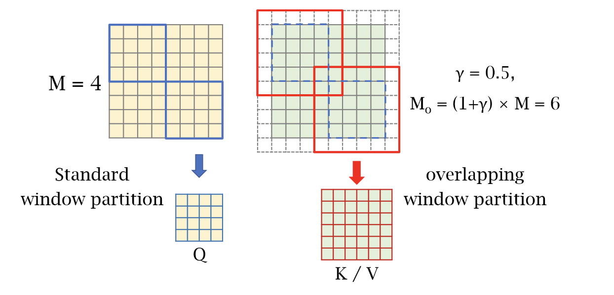
Fig 4. The overlapping window partition for OCA [1].
OCAB modules are used throughout the HAT to further allow for cross-window connections; the basic idea is that windowed self-attention is performed on the input as normal, in the exact same manner as in the HAB module, though the windows for the keys and values, while still centered on the same locations as the windows of the queries, are larger than those of the queries, allowing each window to pull in some information from neighboring windows that it normally would not see.
Specifically, for input features \(X\), let \(X_Q, X_K, X_V \in \mathbb{R}^{H \times W \times C}\). \(X_Q\) is partitioned into \(\frac{HW}{M^2}\) non-overlapping windows of size \(M \times M\). \(X_K\) and \(X_V\) are partitioned into \(\frac{HW}{M^2}\) overlapping windows of size \(M_o\times M_o\), where \(M_o\) is calculated as
\[M_o = (1 + \gamma)M,\]where \(\gamma\) is a hyperparameter introduced in order to control the size of the overlapping windows, and the input is zero-padded to account for this larger window. Aside from shifting windows, this allows for even more cross-window information transmission, as each query window, which are the standard size, can pull in information from the key and value windows that include the query window and extend into the space that would otherwise be a separate, independent window. OCAB is specifically designed to mitigate the blocking artifacts that the standard Swin Transformer produces:
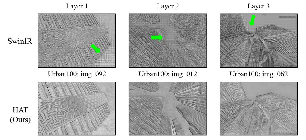
Fig 5. Comparison of blocking between SwinIR and HAT [1].
The OCAB combats this by directly stepping over the hard boundaries between windows, reducing their presence in the extracted features; each query window has access to information about the space beyond its own boundaries, so they can better create smooth boundaries in the features between adjacent windows. While standard window shifting has a similar goal, each shifted window still only has access to its own pixels, which may still lead to hard boundaries and blocking between windows that become present in the features.
Empirically, \(\gamma=0.5\) was found to give the best performance, translating to overlapping windows that are, by area, 4/9 composed of the original window and 5/9 composed of adjacent windows. This is less extreme than the shifted windows of the standard Swin Transformer, where, since the regular shifting amount is half of the window size in each dimension, shifted windows are only 1/4 composed of their original window, and are 3/4 composed of other windows. Still, this additional method of cross-window attention gives the model greater flexibility and another opportunity to use a larger portion of the original image in its reconstruction process.
Residual Hybrid Attention Group (RHAG)
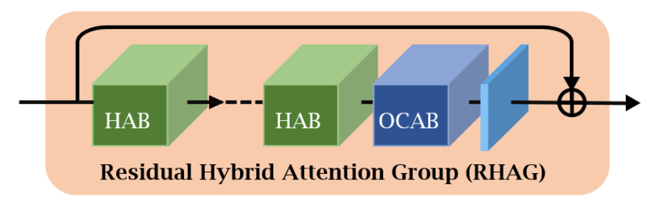
Fig 6. The structure of a Residual Hybrid Attention Group [1].
These modules are combined in a further modular format via a Residual Hybrid Attention Group (RHAG), which puts a variable number of HAB modules in sequence which are followed by an OCAB module, with a final convolutional layer to ensure compatability between shapes of the input and output that allows for a residual connection over the entire module. The sequencing of HAB modules mirrors the structure of standard Swin stages, as the attention windows are shifted between subsequent HABs; though, patch merging is skipped in favor of the OCABs, as they both aim to combine information between windows, and OCAB can retain the spatial size of the input.
High-Level Model Structure
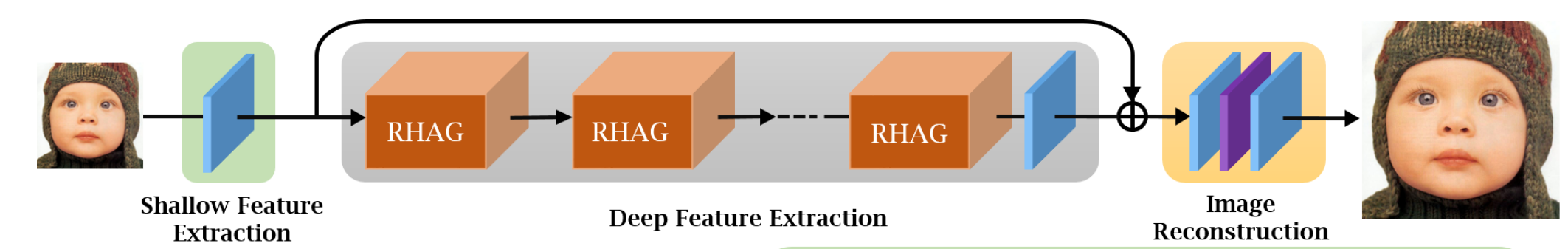
Fig 7. The high-level structure of the HAT [1].
Contrary to the standard Swin, projection to the desired channel dimension is done using an initial convolutional layer; though, mirroring the structure of the Swin Transformer, multiple RHAG modules are placed in sequence (similar to the sequence of stages in Swin), though in this case, a residual connection (along with a convolutional layer to ensure compatability of shapes) is employed across the series of RHAGs. Then, the final image reconstruction is performed using convolutions (for channel number adjustments) and pixel shuffle, where pixels from many channels are pulled together sequentially into a smaller number of channels with a larger image size.
Results
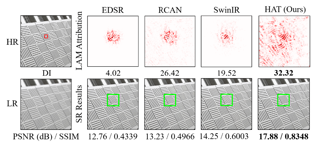
Fig 8. LAM results for different SR methods [1].
In practice, the HAT does, indeed, use a larger portion of the input image for reconstruction than other Transformer-based SR methods. Above is a comparison of Local Attribution Maps (LAM) between different models, which is a method for measuring which portions of the input were most influential for a given patch of the output. We see that HAT is highly nonlocal compared to other methods in terms of LAM, and performs better for it.
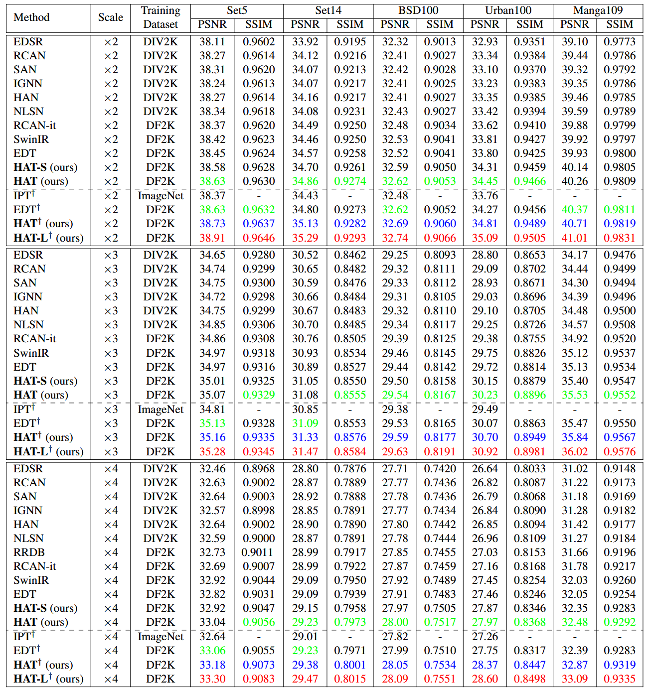
Fig 9. Quantitative results for HAT compared to other methods [1].
The authors compared 3 versions of the model: HAT-S, HAT, and HAT-L: HAT has a similar size to the existing Swin super-resolution model SwinIR, with 6 RHAG modules with 6 HABs each; HAT-L is larger than HAT, with 12 RHAGs instead of 6; HAT-S is smaller than HAT, utilizing only depthwise convolutions and featuring a smaller channel number throughout the model, resulting in overall computation similar to that of SwinIR. Quantitatively, in terms of peak signal-to-noise ratio (PSNR) and structural similarity index measure (SSIM), two standard metrics for image reconstruction, HAT’s variants outperform their peers (if only slightly), and larger HAT models tend to yield better performance (again, if only slightly).
Conclusion
The HAT is a notable modification of the Swin Transformer architecture, designed for super resolution, due to its large practical receptive field; while all SR methods have an entire image to work with as input, it takes effort and specific design to actually use the information that is there in an efficient manner, which can be crucial to reconstructing an image correctly. Judging by its quantitative results, the future state-of-the-art in SR will likely be driven, to some degree, by the development of methods that are designed to produce even larger receptive fields. However, due to the large, Transformer-based architecture, despite using the Swin Transformer, the larger HAT variants can be computationally demanding; while the results are favorable, further developments may be required to make a model like this practical.
Look-Up Table (LUT) Methods
There have been relatively few attempts to make modern deep learning-based methods of super-resolution computationally efficient enough for common consumer applications such as cameras, mobile phones, and televisions. Look-Up Table (LUT) methods, as described in [3], aim to bridge this gap by using a precomputed LUT, where the output values from a deep SR network are stored in advance; during inference, the system can quickly retrieve these high-resolution values by querying the LUT with low-resolution input pixels.
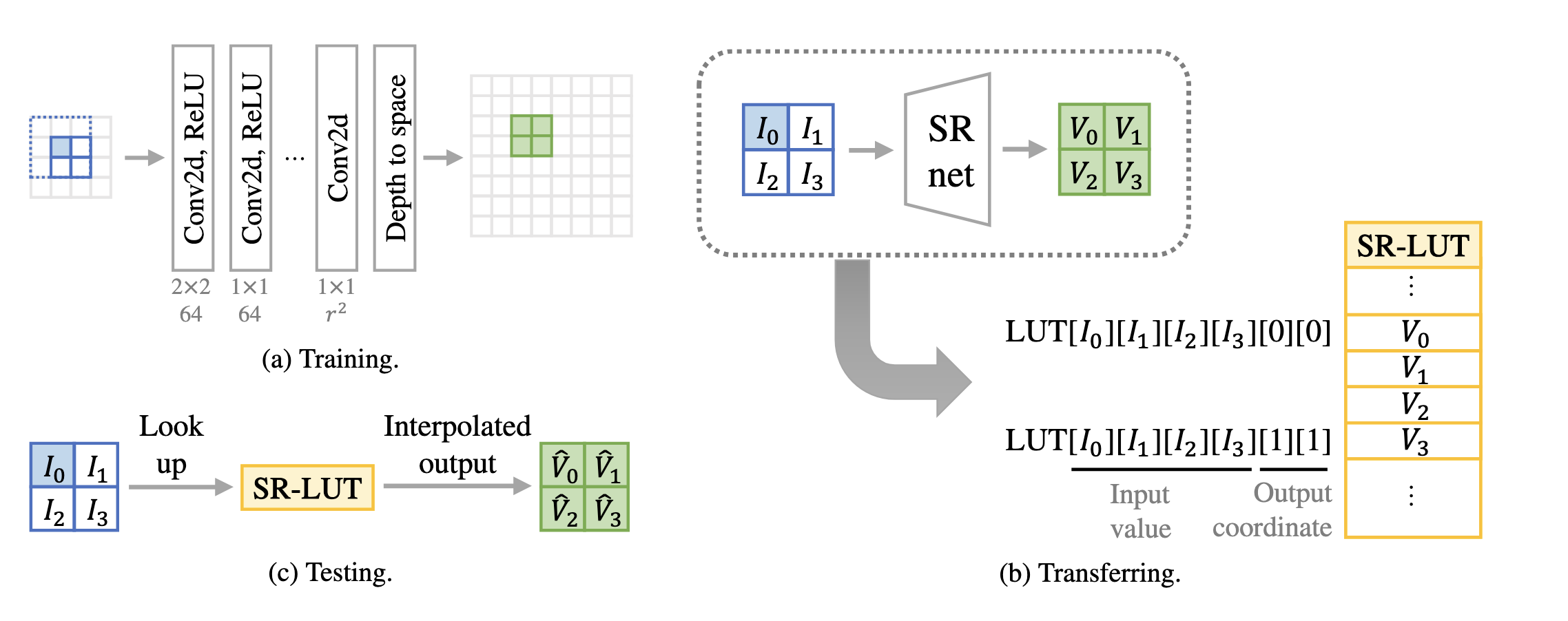
Fig 10. LUT Method Overview [3].
The LUT
It may be useful to start with how the LUT will be used in inference: given a low-resolution image and an upscaling factor \(r\), our goal is will be to map each pixel of the low-res image to an image patch of size \(r \times r\), which we then assemble into a full upscaled image. This process will be done independently for each color channel, so that we are assembling 3 independent images with 1 color channel each and then concatenating them to form a 3-channel image. For a given image pixel at location \((i, j)\), we would like this mapping to take into account the pixels surrounding \((i, j)\) as well as the pixel itself; so, to get the patch for pixel \((i, j)\), the LUT will be indexed by a fixed number of pixel values surrounding \((i, j)\) (given that we use pixel values for indexing, we use 8-bit color), and at this index in the LUT, there will be \(r^2\) values that we can use to construct an image patch. For instance, for \(r=2\) and a LUT receptive field of 4, let \(I_0 = image[i, j], I_1 = image[i+1, j], I_2 = image[i, j+1], I_3 = image[i+1, j+1]\). Then, \(LUT[I_0][I_1][I_2][I_3][0][0]\) will contain the top-left corner of the upscaled patch, and \(LUT[I_0][I_1][I_2][I_3][1][1]\) will contain the bottom-right corner. This will be the basic method that the LUT uses in inference, which only requires table lookup, and no network computation.
The SR Network
Now, with a clear goal of how the LUT should function, we can construct the network that will give us its values. Given that we want the patch in the LUT for each specific pixel value to depend solely on a fixed number of surrounding pixels, a convolutional network with a finely-controlled receptive field seems natural; again, note that the LUT upscaling process is performed independently on each color channel, so the input to this network will only have 1 channel. Specifically, given a receptive field size \(n\) and an upscaling factor \(r\), we can construct a network as:
-
a series of convolutional layers (with nonlinearities), where, at the end, each output pixel has a gross receptive field of size \(n\) and the output has \(r^2\) channels
-
a pixel shuffle that will construct upscaled patches from our channels and concatenate them together into a full upscaled image
with this, we have constructed a network where each tiled \(r \times r\) patch of the output depends only on a (contiguous) size \(n\) receptive field from the input. Now, if we optimize this network for super-resolution, to construct our LUT, we can simply generate patches of size \(n\) with specific values (which will be indexes in the LUT) and feed them into the network, and the resulting upscaled patch can be added to the LUT at the given index. The kernels of the convolutional layers could be anything as long as it conforms to the receptive field requirement, however, the authors of the paper use an architecture where the first convolutional layer results in a receptive field of size \(n\), and all subsequent layers are \(1\times 1\) convolutions (the issue of the kernel reducing the size of the input is dealt with by pre-padding the image); additionally, they use a square kernel when possible, as it will capture the pixels that are most adjacent, and thus most relevant, to each other, compared to a non-square kernel.
LUT Size
Of course, the principal design priority of the LUT is efficiency in speed and size. Using 8-bit color, if we construct a LUT that accounts for every possible input patch, one can compute the size of the LUT for a given receptive field \(n\) and upscale factor \(r\) as
\[(2^8)^n r^2 \text{ bytes}\]This can be seen clearly from the structure of the LUT; there are \(2^8\) possible values for a given 1-channel pixel (again, for 8-bit color), so for a RF of size \(n\), there are \((2^8)^n\) possible input patches. At each index corresponding to an input patch, there is an upscaled patch of size \(r^2\), whose entries are also each 8 bits (or 1 byte). Clearly, this will not scale well with \(n\), and in fact, \(n=4\) and \(r=2\) gives us a LUT that is 16GB large. To counteract this, [3] uses a “sampled LUT”, where only a subset of the possible input patches are sampled for use in the LUT; specifically, they found that sampling the color space of \(0\) to \(2^8-1\) uniformly (including endpoints) with a sampling interval of \(2^4\) over each pixel of the input patch worked well to reduce the size of the LUT while retaining good performance, reducing the 16GB LUT to just \((1+\frac{2^8}{2^4})^4 2^2 = 334084\) bytes, or about 326KB.
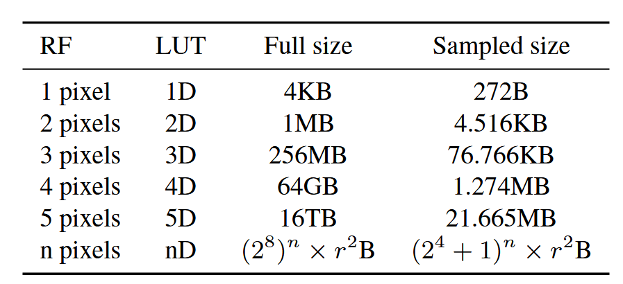
Fig 11. A comparison of LUT sizes for \(r=4\) [3].
Of course, this sampled LUT introduces the issue of indexing: how do we index from the LUT if the input patch doesn’t match a patch that was seen while filling out the table? For this, the authors used interpolation; instead of indexing one upscaled patch, we can interpolate between up to \(2^n\) patches, for a RF size \(n\). For instance, for a LUT where \(n=2\), using a sampling interval of \(2^4\), getting the upscaled patch for an input patch where \(I_0 = 8, I_1 = 8\) would require interpolating between \(LUT[0][0], LUT[0][1], LUT[1][0], LUT[1][1]\). Using this sampling interval, these nearest points can actually be found easily by looking at the bit representation of \(I_j\): the first 4 bits, when converted to integer, will be the index of the lower part of the interpolation (e.g. for \(I_j = 20\), 20 \(\to\) 00010100, and then 0001 \(\to\) 1, meaning that \(LUT[1]\) will be the lower part of the interpolation and \(LUT[2]\) will be the upper part); this method of indexing for the interpolation points adds even further to the LUT’s speed. The issue of interpolating between points in \(n\) dimensional space is complex in its own right, though we note that the authors found that linear interpolation was slower than triangular interpolation (and its higher-dimensional couterparts), especially for larger \(n\).
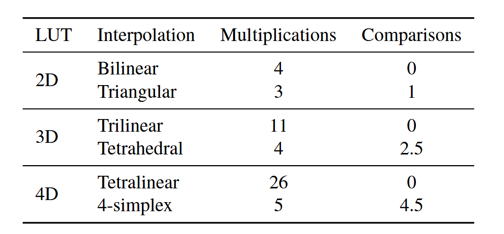
Fig 12. A comparison of interpolation methods for \(n=2, 3, 4\) [3].
Rotational Ensemble
Additionally, during training and testing, the authors employed the strategy of “rotational ensemble”. This is a method of data augmentation that involves:
-
rotating each input by 90, 180, and 270 (and 0) degrees
-
feeding each of the 4 rotations of the input into the model
-
rotating each the super-resolution outputs such that they are all at their original orientation
-
taking the average over the 4 outputs, and treating that as your final output
This method is well-suited to our task; images that are rotated still fall under our base assumption of what “real” images look like for super resolution, so the model can improve by optimizing over them. In our case, this method can actually improve the effective receptive field of the model substantially:
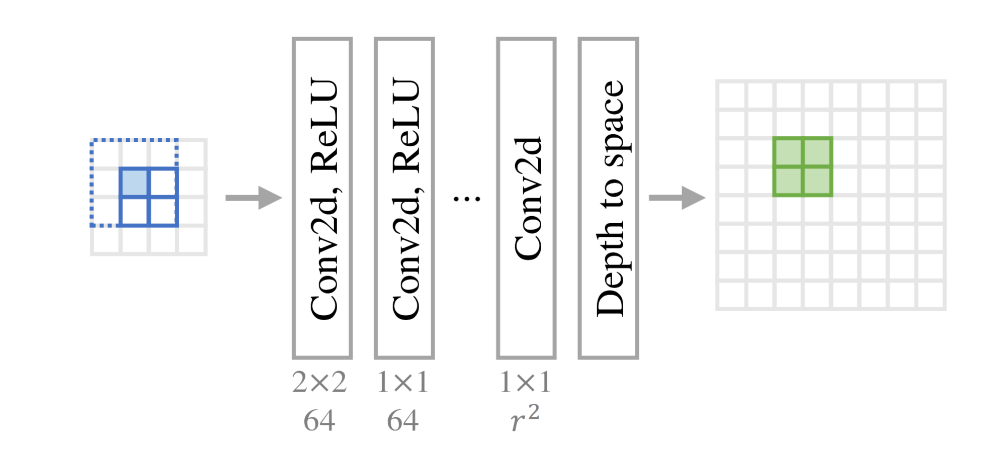
Fig 13. An illustration of the effect of rotational ensemble on the receptive field; a 2x2 RF is effectively increased to a 3x3 RF [3].
During training, rotational ensemble simply works well as a way to increase your dataset size. However, this method can be used in inference as well; we can construct 4 different super-resolution predictions using the LUT, and then average them together. For a 2x2 square RF, one can see, in the illustration above representing 2x upscaling, that the relative position of the patch in the output corresponding to the RF in the input will be determined by the relative position of the top-left pixel of the RF in the input image; that is, any RF in the input, no matter the rotation of the image, will correspond to the same patch in the output as long as the top-left pixel of the RF is the same across those RFs in the input. So, when we look at the RFs across our rotational ensemble when the top-left pixel is kept constant, we see that their union will be a 3x3 area in the input, which means that the given output patch will be influenced by all pixels in the 3x3 area, effectively increasing our inference RF size to 9.
While this does increase our inference computation time by a factor of 4 (discounting rotations and averaging), it is likely a worthy trade-off for such a substantial increase in RF size, which would normally require increasing the LUT size to an unmanageable degree.
Results
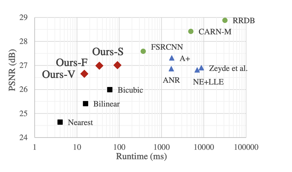
Fig 14. Peak signal-to-noise ratio (PSNR) and runtime of various methods for 320 x 180 -> 1280 x 720 upscaling [3].
There are 3 models mentioned in the paper: V, F, and S, which have a receptive field of 2, 3, and 4, respectively. F and S use a sampled LUT with a sampling interval of \(2^4\), while V uses a full LUT. We see that the LUT methods provide a good tradeoff in terms of speed vs reconstruction quality, where F is even faster than bicubic interpolation, and V is even faster than bilinear interpolation.
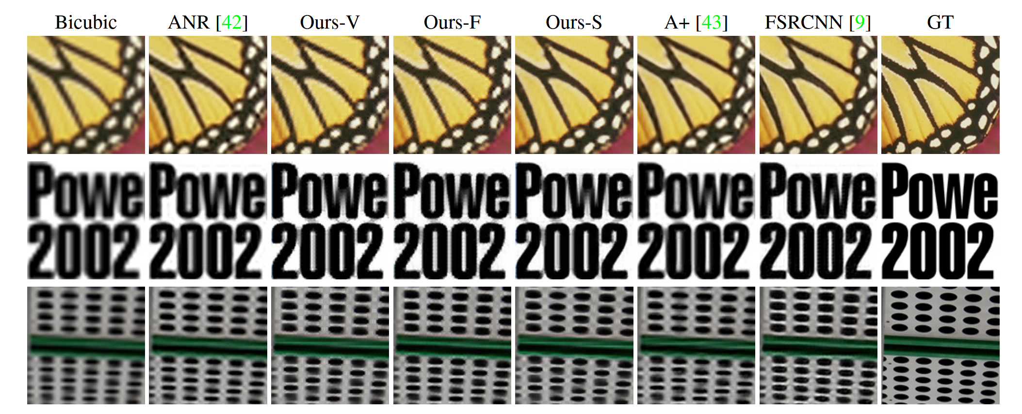
Fig 15. Qualitative comparison of results [3].
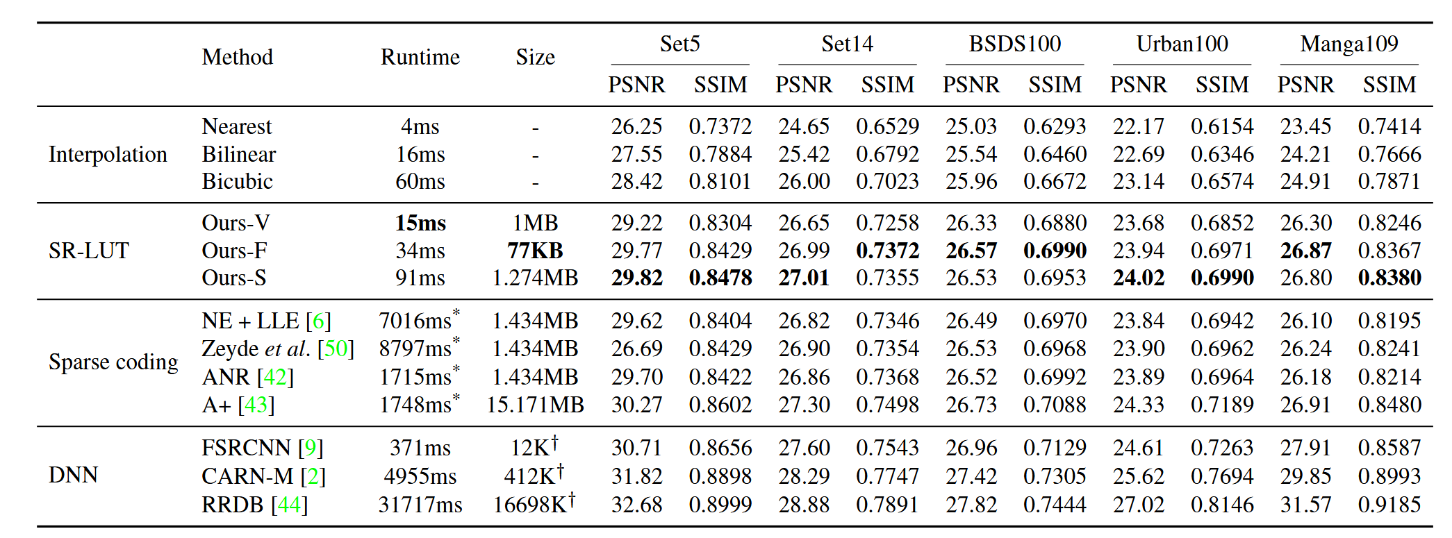
Fig 16. Quantitative comparison of results; runtimes for all methods besides sparse coding are on a Galaxy S7 phone [3].
We see that, quantitatively, all LUT variants perform substantially better than traditional interpolation upscaling methods, and are competitive with methods that require far greater runtime and/or storage space. Interestingly, there are some cases where the F model seems to perform quantitatively better than the S model, despite the fact that the only difference between them is that S has a larger receptive field. This likely just indicates a plateau in performance wrt receptive field size, or the differently shaped receptive fields may fare differently on different datasets (since RF=3 for F and RF=4 for S, the RF for F is a line and the RF for S is a square).
LUT methods are an interesting way to make super-resolution more efficient; instead of making a more efficient network, it avoids using a network for inference altogether. However, there are some obvious flaws: the quantitative results do not make it state-of-the-art in that regard, and the methodology of using the same LUT for each color channel independently seems somewhat unintuitive. Additionally, a given LUT is confined to a fixed receptive field size and upscaling factor; an entirely new SR network and table must be created to change these factors, which restricts the method’s practical use.
IM-LUT
Since its invention in 2021, there have been numerous published papers for extensions and modifications to the LUT. One of these, published in 2025, is Interpolation Mixing LUT, or IM-LUT [5]. IM-LUT allows for the model to adapt to the scaling factor at inference time, meaning that a single IM-LUT can be used to scale any image to any size. This is achieved by first upscaling the input image with standard interpolation algorithms, such as bicubic upsampling, and then using a standard LUT on the upscaled image. However, the IM-LUT can also adapt its interpolation to the input image dynamically; a single IM-LUT first uses many different interpolation algorithms, and then uses a weighted average, with weights based on the image itself and the given scale factor, to combine the interpolations together before the final refinement LUT. With this, the IM-LUT can adapt to any scaling factor while still also dynamically adapting to the specific input image.
Now, we go through the structure of the IM-LUT.
IM-Net
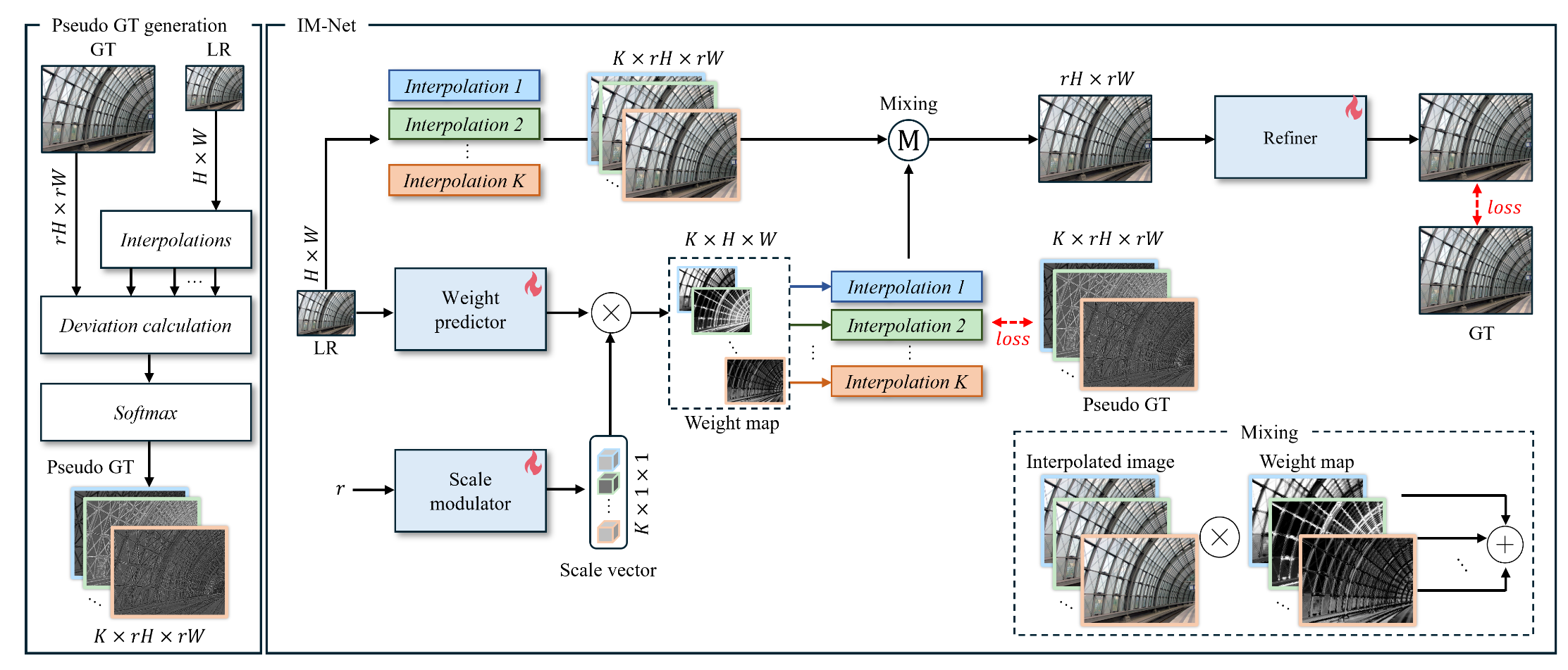
Fig 17. IM-Net, the network used to generate the LUTs for IM-LUT [5].
There are two overall parts to the IM-Net: weight map prediction, and image refinement. Image refinement is simply a network that refines an the interpolated input image; it takes an image of any given size, and produces an image of the same size. This part of the network is simple, but the weight maps are more involved:
The IM-LUT works with a fixed set of \(K\) interpolation functions, and for any given image, the network predicts per-pixel weights for each interpolation function; these weight maps allow the network to take advantage of the fact that different interpolation methods may fare better in different areas of a given image. The weight maps are a combination of the output of two other networks:
-
An image-to-weight map network, that takes the low-resolution image and produces low-resolution weight maps.
-
An upscaling factor-to-scale vector network (“scale modulator”), that takes the scaling factor as input and outputs a vector of per-interpolation function weights.
The weights from the scale modulator are multiplied by the initial weight maps (one scale weight per weight map) to produce the final weight maps. The networks optimize their predictions of these weight maps as so:
-
For a given image (where the ground truth is known) and upscaling factor, downscale the image and then get interpolations back to the original size using each given interpolation function.
-
Calculate per-interpolation deviations from the GT image using per-pixel L1 loss, i.e. \(E_k[i, j] = |\hat I_k[i, j] - I_{\text{GT}}[i, j]|\) for \(k=1,...,K\).
-
Compute ground-truth weight maps as a temperature-controlled per-pixel softmax over all negative interpolation deviations, i.e. \(W^{GT}_k[i, j] = \frac{e^{-\beta E_k[i, j]}}{\sum_{\ell=1}^K e^{-\beta E_\ell[i, j]}}\) for \(\beta\) being the temperature constant.
-
Compute the “guide” loss (or, the weight map loss) as the L2 reconstruction loss between the predicted and ground-truth weight maps, that is \(\mathcal{L}_{\text{guide}} = \sum_{\ell=1}^K ||\hat W_\ell - W^{GT}_\ell||_2\)
Then, when the predicted weight maps are used to create a final interpolated image, and that is run through the refinement network, the final reconstruction loss can be found as \(\mathcal{L}_{\text{rec}} = ||\hat I - I^{GT}||_2\) and the final loss that we optimize over is \(\mathcal{L} = \mathcal{L}_{\text{rec}} + \lambda \mathcal{L}_{\text{guide}}\) where \(\lambda\) is our trade-off hyperparameter. With this, we can optimize both the refinement and the weight map predictions at once, and we can vary the upscaling factor to ensure that the network can adapt well to different amounts of upscaling.
IM-LUT
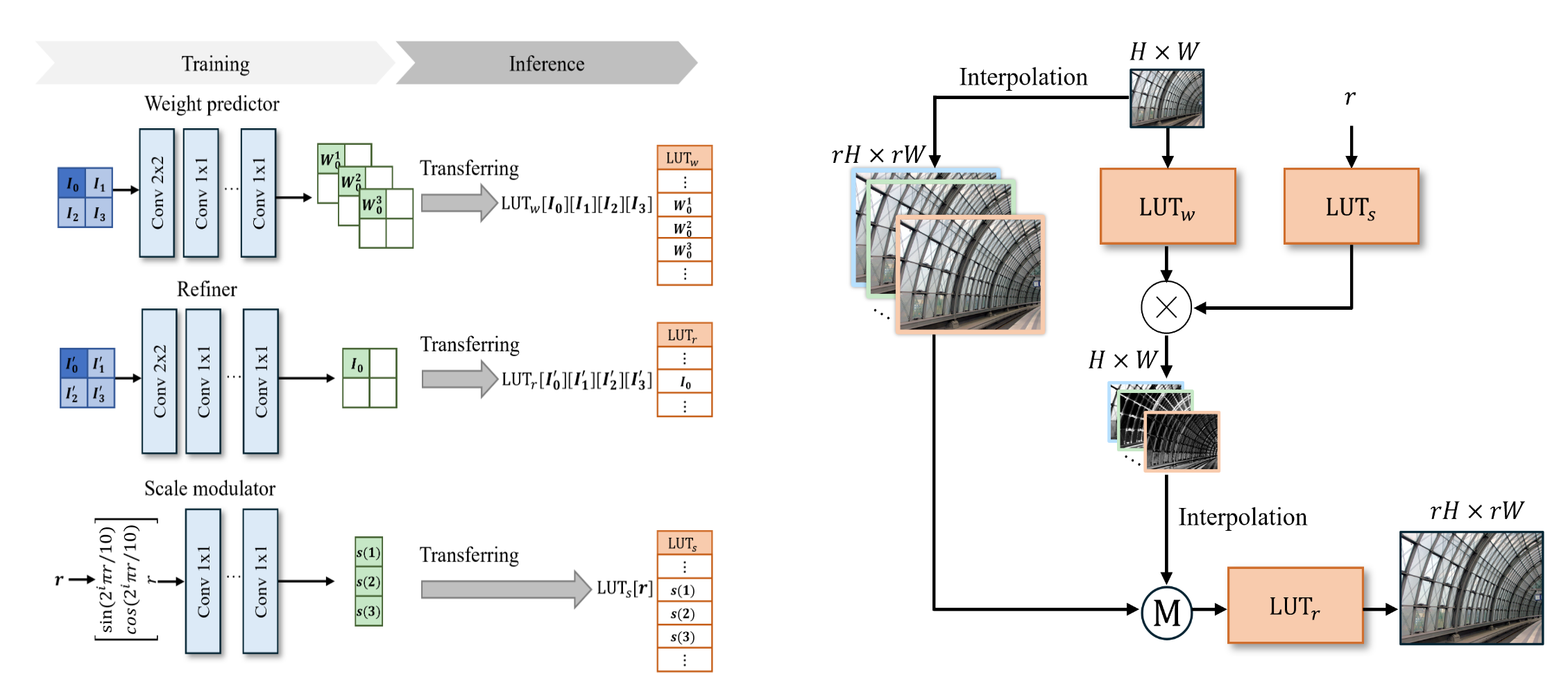
Fig 18. An overview of the way in which the LUTs are created and used [5].
Now, we have to transfer the IM-Net to LUTs. Given that IM-Net has 3 distinct sub-networks (scaling factor network, weight map network, and refinement network), we will have 3 LUTs; note that the refinement and weight map networks each use convolutional networks that leave each pixel of the output with a 2x2 receptive field in the input, as was seen with the original LUT. Additionally, each LUT is created with a sampling-interval scheme and interpolated indexing, as was also seen with the standard LUT (except for the scale LUT, which uses nearest neighbor interpolation). Specifically, the scale modulator LUT is indexed by a single number and outputs a vector of \(K\) weights, making it small and efficient; the weight map LUT is indexed by 4 pixel values and outputs \(K\) pixel values (since the weight map network does not perform any resizing), making it similar in size to the standard LUT; the refiner LUT is indexed by 4 pixels and outputs 1 pixel value (again, no resizing), making it smaller than the standard LUT. We see that, unlike the standard LUT, the size of the LUTs has no dependence on the scale factor; however, given that the refiner LUT will be used on the entire upscaled image, the overall computational complexity will increase with the scale factor (though, as noted in [5], it does not increase substantially).
Once the LUTs are computed, they can be used as stand-ins for the networks (as in the standard LUT), and then images can be upscaled as they were in IM-Net.
Results
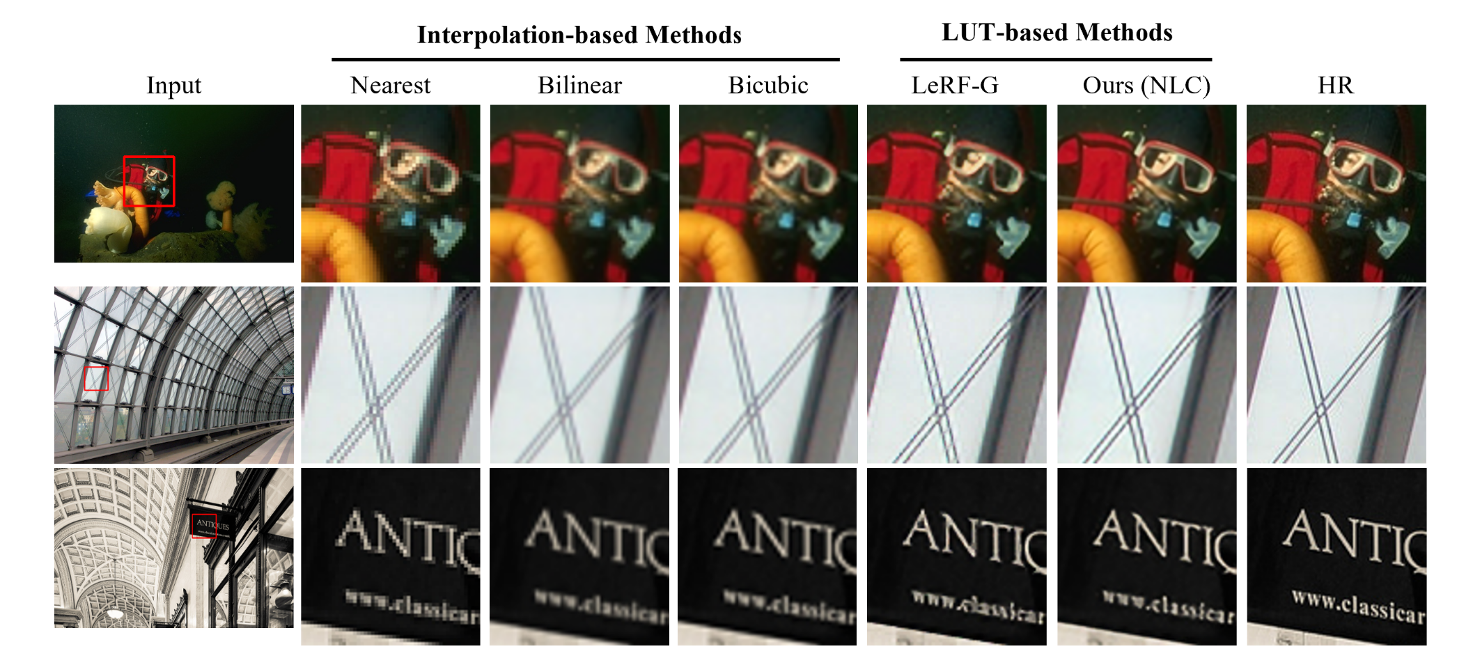
Fig 19. Qualitative results of IM-LUT compared to other methods [5].
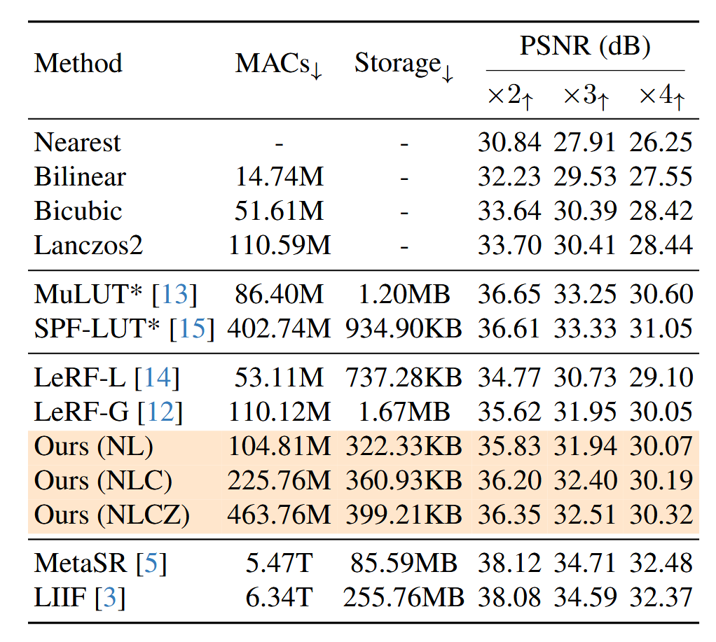
Fig 20. Multiply-accumulate (MAC) operations, required storage, and PSNR for various super-resolution methods [5].
Given the freedom to choose interpolation functions, the authors highlight a few possible combinations of functions: in the table above, N means “nearest neighbor”, L means “bilinear”, C means “bicubic” and Z means “lanczos”, another kind of interpolation algorithm that uses windowed normalized sine functions; the letters, when put together, indicate that the given IM-LUT uses all of those interpolation functions. We see that the IM-LUT methods manage to be very efficient on storage and, for certain combinations of interpolations, on computations, as well; at the same time, they have much better performance than any single interpolation function, and, while not being state-of-the-art quantitatively, stay competitive with other LUT or similarly-efficient SR methods that require more storage and, in the case of the other LUT methods, cannot use a single model to adapt to different scaling factors.
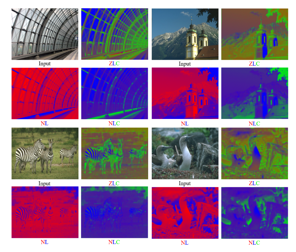
Fig 21. Analysis of weight maps for different interpolation functions [5].
From the color-coded weight maps above, we see that the model is, in fact, using the weight maps to adapt to the input image. For instance, when nearest-neighbor and bilinear interpolation are used together, we see that the bilinear interpolation is prioritized in areas of low brightness, while the nearest neighbor method is used elsewhere. However, we also see that when nearest-neighbor, bilinear, and bicubic interpolation are used together, the nearest-neighbor interpolation has very little influence, indicating that one could even use the weight maps as a form of interpolation function selection, similar to how L1 regularization is used as variable selection in linear regression.
Conclusion
The IM-Net is already an interesting kind of reparameterization of the problem of learning-based super-resolution; instead of directly learning how to upscale an image, the network instead learns how to ensemble a set of given interpolation functions to do upscaling. This modular design allows for a great deal of flexibility in the model, as it can be combined with any arbitrary-scale upscaling method, even other learning-based methods, without any change to the core architecture. Of course, in this case, our real goal is a LUT-based method; in the realm of LUT-based methods, IM-LUT still stands out for its capability of arbitrary-scale super-resolution. Dynamically adapting to different scales will be a practical necessity for any super-resolution method, so it will be interesting to see if, as time goes on, efficient super-resolution methods will expand further in the direction of the IM-LUT, or if an entirely different architecture will rise to the top; the obvious downside of LUT methods is their low accuracy, so it will be especially noteworthy if a whole new kind of model structure can improve on this while retaining the benefits of LUT and allowing for arbitrary scales.
Unfolding Networks
The “unfolding” in “unfolding network” refers to splitting up the problem of image reconstruction into two distinct subproblems, that being (1) deblurring and upsampling, and (2) denoising. With this approach, one can show that problem (1) has a closed-form optimal solution that can explicitly adapt to specific given types of degradation with 0 learned parameters; this greatly reduces the burden on the learned portion of the network, which now only needs to do denoising. The method is a kind of fusing of model-based and learning-based approaches; despite involving a variant of a UNet, it is designed to be zero-shot adaptable to any kind of degradation that is parameterized by a known blurring kernel, downsampling factor, and noise level.
Now, we can go through and derive the method ourselves to illustrate how it arises:
Derivation
The basic assumption will be that the input image for the method will be the blurred, downsampled, and additive white Gaussian noise-ed version of a ground-truth image, or in other words, our degraded image \(\vec y\) is
\[\vec y = (\vec x \otimes \vec k)\downarrow_s + \vec N\]where:
- \(\vec x \otimes \vec k\) represents the application of blurring kernel \(\vec k\) to ground-truth image \(\vec x\) (via convolution)
- \(\downarrow_s\) represents downsampling (decimation) by a factor of \(s\)
- \(\vec N \sim N(\vec 0, \sigma^2 I)\) for noise level \(\sigma \in \mathbb{R}^+\)
Given that \(\vec y \sim N((\vec x \otimes \vec k)\downarrow_s, \sigma^2 I)\), its PDF is
\[P(\vec y | \vec x) = \frac 1 {(2\pi\sigma^2)^{\frac p 2}}e^{-\frac 1 {2\sigma^2}||(\vec x \otimes \vec k)\downarrow_s - \vec y||_2^2}\]Furthermore, it will be useful to have an image prior, which we will define as
\[\Phi(\vec x) = -\log P(\vec x)\]which will stand as a measure of how “natural” an image \(\vec x\) is, ideally being minimised for any of our ground truth images and being maximised for images that are very noisy or unrealistic (i.e. unlike our GT images); we could interpret it simply as the negative logarithm of the a-priori probability distribution function of our ground truth images. In a practical sense, incorporating such a measure in our optimization will push our model toward creating images that conform to the patterns that typically appear in real images regarding color, brightness, etc, as opposed to overfitting on an image reconstruction loss function (in other words, a form of regularization).
Now, under a maximum a-posteriori (MAP) framework, our goal in super-resolution, given a degraded image \(\vec y\) conforming to the assumptions above, can be defined as finding
\[\hat x = \arg \max_{\vec x} P(\vec x | \vec y) \\\]Or, in other words, the clean image that the degraded image most likely started as. From Bayes theorem, we have
\[P(\vec x | \vec y) = \frac{P(\vec y | \vec x)P(\vec x)}{P(\vec y)} \propto P(\vec y | \vec x)P(\vec x)\]Since \(P(\vec y)\) is constant with regard to \(\vec x\). So now,
\[\begin{aligned} \hat x &= \arg \max_{\vec x} P(\vec x | \vec y) \\ &= \arg \max_{\vec x} P(\vec y | \vec x)P(\vec x) \\ &= \arg \min_{\vec x} -\log(P(\vec y | \vec x)P(\vec x)) = \arg \min_{\vec x} -\log P(\vec y | \vec x) - \log P(\vec x) \\ &= \arg \min_{\vec x} -(\log(\frac 1 {(2\pi\sigma^2)^{\frac d 2}}) - \frac 1 {2\sigma^2}||(\vec x \otimes \vec k)\downarrow_s - \vec y||_2^2) + \Phi(\vec x) \\ &= \arg \min_{\vec x} \frac 1 {2\sigma^2}||(\vec x \otimes \vec k)\downarrow_s - \vec y||_2^2 + \Phi(\vec x) \end{aligned}\]Additionally, for practical reasons, we often include a “trade-off” hyperparameter, which we represent with \(\lambda\), to balance the influence between our prior term \(\Phi\) and our data term \(||(\vec x \otimes \vec k)\downarrow_s - \vec y||_2^2\) , so we have
\[\hat x = \arg \min_{\vec x} \frac 1 {2\sigma^2}||(\vec x \otimes \vec k)\downarrow_s - \vec y||_2^2 + \lambda\Phi(\vec x)\]Instead of directly minimizing this expression with something like gradient descent, one can actually notice that \(\arg \min_{\vec x} ||(\vec x \otimes \vec k)\downarrow_s - \vec y||_2^2\) has a closed form solution (which we will detail later); so, to take advantage of this fact, we can decouple the data term and prior term in our optimization by using half-quadratic splitting, where we introduce an auxiliary variable \(\vec z\) into our optimization:
\[\min_{\vec x, \vec z}\frac 1 {2\sigma^2}||(\vec z \otimes \vec k)\downarrow_s - \vec y||_2^2 + \lambda\Phi(\vec x) + \frac \mu 2 ||\vec x - \vec z||_2^2\]Now, \(\mu\) is a hyperparameter controlling how much leeway we want to give \(\vec x\) and \(\vec z\) to be different, where \(\mu \to +\infty\) recovers our original problem. Now, given that we have two optimization variables instead of just one, we can unfold the target and perform alternating iterative optimization (with \(j\) as the step number):
\[\begin{aligned} \vec z_j &= \arg \min_{\vec z} \frac 1 {2\sigma^2}||(\vec z \otimes \vec k)\downarrow_s - \vec y||_2^2 + \frac \mu 2 ||\vec x_{j-1} - \vec z||_2^2 \\ \vec x_j &= \arg \min_{\vec x} \lambda\Phi(\vec x) + \frac \mu 2 ||\vec x - \vec z_j||_2^2 \end{aligned}\]Now, it may be useful to change the value of \(\mu\) throughout our optimization; a small \(\mu\) near the start of our optimization will help speed up convergence, and a large \(\mu\) near the end will ensure that our solution actually corresponds to the original problem. So, define \(\mu_1, ..., \mu_J\) for an optimization of \(J\) steps, and let \(\alpha_j = \mu_j\sigma^2\), so we have
\[\begin{aligned} \vec z_j &= \arg \min_{\vec z} ||(\vec z \otimes \vec k)\downarrow_s - \vec y||_2^2 + \alpha_j ||\vec x_{j-1} - \vec z||_2^2 \\ \vec x_j &= \arg \min_{\vec x} \Phi(\vec x) + \frac {\mu_j} {2\lambda} ||\vec x - \vec z_j||_2^2 \end{aligned}\]Now, as alluded, \(\vec z_j\) actually still has a closed form solution:
\[\vec z_j = \mathcal{F}^{-1} \left(\frac{1}{\alpha_j}\left(\vec d - \overline{\mathcal{F}(\vec k)} \odot_s \frac{(\mathcal{F}(\vec k)\vec d) \Downarrow_s}{(\overline{\mathcal{F}(\vec k)}\mathcal{F}(\vec k))\Downarrow_s + \alpha_j} \right) \right)\]where
\[\vec d = \overline{\mathcal{F}(\vec k)}\mathcal{F}(\vec y \uparrow_s) + \alpha_j \mathcal{F}(\vec x_{j-1})\]and \(\mathcal{F}\) denotes the discrete FFT (and \(\mathcal{F}^{-1}\) is the inverse discrete FFT), \(\odot_s\) is the distinct block processing operator with element-wise multiplication, \(\Downarrow_s\) denotes the block downsampler, and \(\uparrow_s\) denotes the upsampler. The derivation of this solution is too long to include here, but is detailed in [4].
So, it remains to find \(\vec x_j = \arg \min_{\vec x} \Phi(\vec x) + \frac {\mu_j} {2\lambda} ||\vec x - \vec z_j||_2^2\). One can notice that this is similar to our very first optimization target; indeed, finding \(\vec x_j\) is equivalent to removing additive white Gaussian noise from \(\vec z_j\) with \(\sigma^2_\text{noise} = \frac {\lambda} {\mu_j}\) under a MAP framework. So, for convenience, we define \(\beta_j = \sqrt{\frac{\lambda}{\mu_j}}\) (the standard deviation of the Gaussian noise), and we have that finding \(x_j\) is equivalent to a Gaussian denoising problem with noise level \(\beta_j\) (or, \(\sigma^2_\text{noise} = \beta_j^2\)).
Given that this is a simple denoising task, we can opt for a denoising neural network.
Denoising Network
The paper in question uses a “ResUNet”, which is a variant of a UNet:
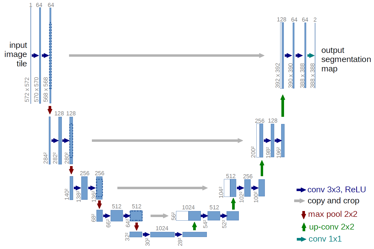
Fig 22. UNet architecture as depicted in [6].
The ResUNet involves four scales, in which 2x2 strided convolutions and 2x2 transposed convolutions are adopted for down- and up-scaling, respectively, and residual blocks with the same structure as from ResNet are added between these size changes; of course, skip connections between downscaling and upscaling are also employed, as in the regular UNet.
In order to ensure adaptibility and nonblind-ness of the method, it is useful to incorporate the noise level \(\beta_j\) into the network input. The method in [2] for doing this is fairly simple: given an input image \(3 \times H \times W\), a constant matrix with size \(H \times W\) with all entries equal to \(\beta_j\) is appended on the channel dimension to create an input of shape \(4 \times H \times W\), which is fed into the network as normal.
Network Modules
Now, to explicitly modularize the method so far, the authors introduce various network modules. First, we have the data module \(\mathcal{D}\), which is used to give us \(\vec z_j = \mathcal{D}(\vec x_{j-1}, s, \vec k, \vec y, \alpha_j)\), which is the optimal solution to
\[\vec z_j = \arg \min_{\vec z} ||(\vec z \otimes \vec k)\downarrow_s - \vec y||_2^2 + \alpha_j ||\vec x_{j-1} - \vec z||_2^2\]Of course, this is achieved with the closed form solution detailed above, so this module has no learnable parameters and can explicitly adapt to any blurring kernel, scale factor and noise level \(\sigma\) (through \(\alpha_j\)).
The prior module \(\mathcal{P}\), which is used to give us \(\vec x_j = \mathcal{P}(\vec z_j, \beta_j)\), is trained to optimize the other objective
\[\vec x_j = \arg \min_{\vec x} \lambda\Phi(\vec x) + \frac \mu 2 ||\vec x - \vec z_j||_2^2\]As alluded, this encapsulates the denoising ResUNet.
Lastly, the hyperparameter module \(\mathcal{H}\) is introduced to allow for dynamic hyperparameter selection. This module takes in the noise level \(\sigma\) and scale factor \(s\) and uses a MLP to predict optimal \(\lambda\) and \(\mu_1, ..., \mu_J\) for the given problem, which can then be used to compute \(\alpha_1, ..., \alpha_J\) and \(\beta_1, ..., \beta_J\).
Overall Model Structure
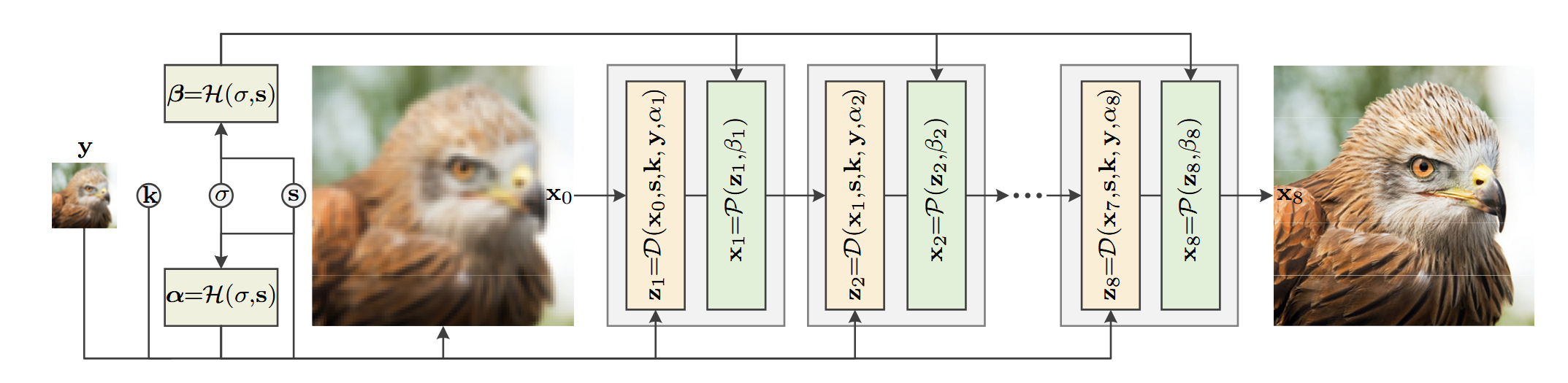
Fig 23. The full architecture of the unfolding network [2].
These modules are combined by first predicting hyperparameters \(\alpha_j\) and \(\beta_j\) through the hyperparameter module, and then stacking the data and prior modules sequentially, performing iterative optimization on the low resolution input image (which is first upsampled with nearest-neighbor interpolation to be the target size before being fed into the network).
With all of this, the authors note that the model is trained in a end-to-end fashion, where scaling factors, blurring kernels, and noise levels are sampled from a pool throughout training to generate LR samples. While certain portions of the network can explicitly adapt to these factors, the denoising network (and hyperparameter module) cannot do so in the same manner, and so varying these values throughout training ensures that the network, as a whole, is robust and adaptable.
Results
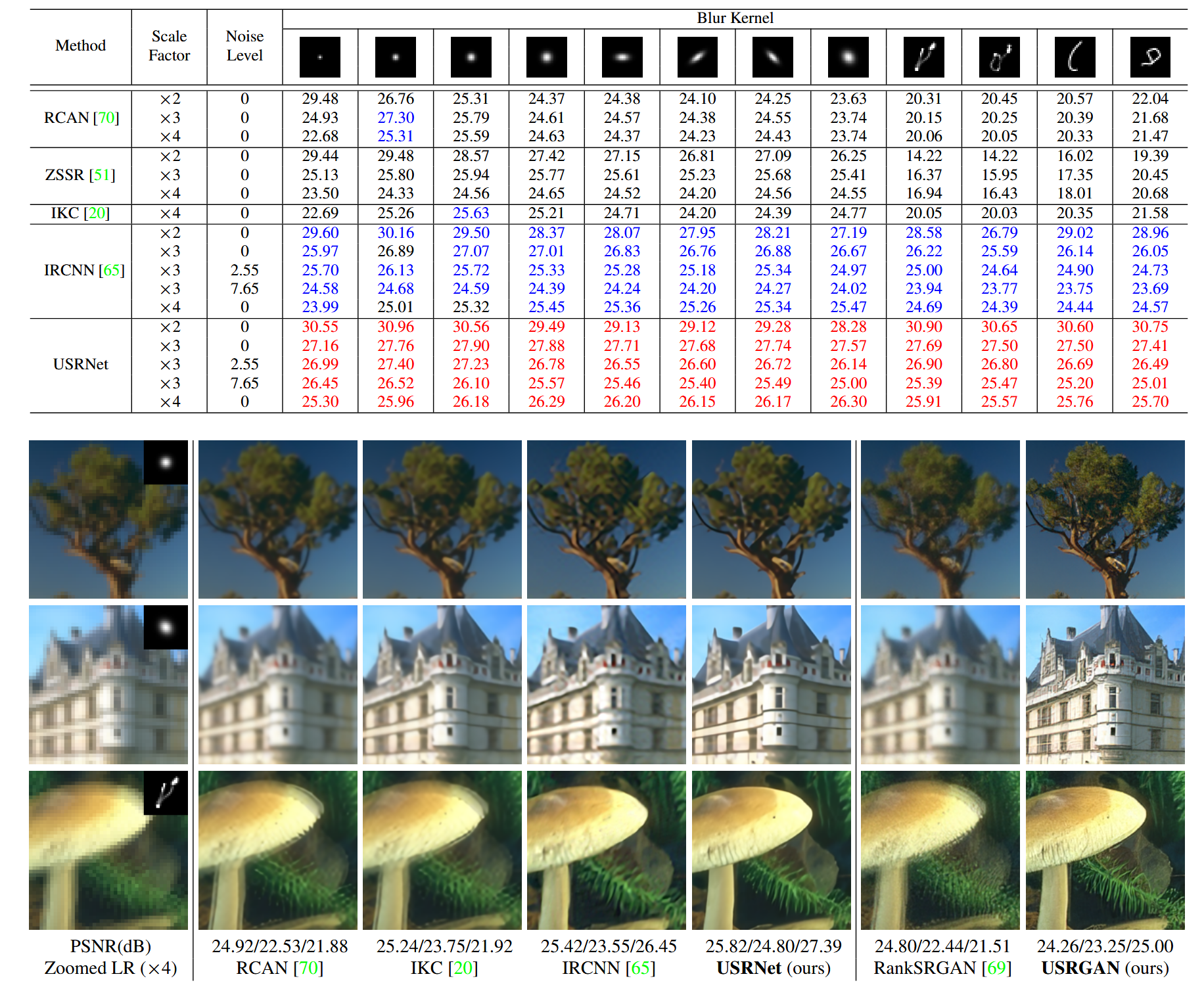
Fig 24. Quantitative and qualitative results of various methods [2].
We see that the unfolding network performs favorably compared to its peers, both qualitatively and quantitatively, for a variety of scaling factors, noise levels, and blurring kernels. Due to the explicit adaptibility to these factors, the model can even be effective even at parsing images that humans may have trouble with:
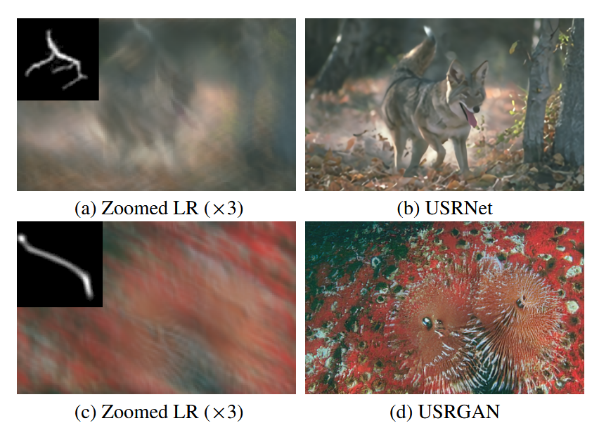
Fig 25. Qualitative results of deep unfolding network with the associated blurring kernels [2].
Conclusion
Of course, in practice, we often may not have much idea about the specific blurring kernel or noise level for our given image, which limits the effective use of this model structure. Additionally, performing denoising only with convolutions, despite the use of a UNet, may limit the method’s effective receptive field.
However, in all, the deep unfolding network is an interesting blend of model-based and learning-based methods; they can both be very useful in their own right, and can empower each other when combined. The efficient, learning-free data module makes the optimization problem of the learned prior module much easier, and attains an optimal solution that could have required many times more parameters to replicate in a learning-based method. Conversely, the prior module can give us an accurate approximation for a complex, statistical problem, which model-based methods can struggle with.
Experiments: An Extension of the Hybrid Attention Transformer
Adaptive Sparse Transformer (AST)
While Transformers have shown immense success in vision tasks due to their ability to model complex, long-range relationships, this can also be a detriment; for reconstructing a given portion of an image, there are likely many parts of the image that are not relevant, and trying to use information from those parts will only add noise to the reconstruction. The self-attention mechanism of the regular Transformer has all tokens attend to all other tokens, with (Softmax) attention weights that will always be greater than 0. While the Transformer can use very small attention scores as a way of giving less attention to irrelevant tokens, it is likely useful to give the model more direct flexibility in selecting relevant image regions that does not require assigning scores of large magnitude; for this, [7] proposes the Adaptive Sparse Transformer (AST).
The AST changes the standard Transformer architecture in two ways: first, instead of just using Softmax on the attention scores to get attention weights, it introduces sparse score selection by using a weighted sum of the Softmax and squared-ReLU of the attention scores to get the attention weights, where the weight between the two schemes is a learnable parameter. With this, our Transformer has both “dense” (Softmax) attention weights, which makes all weights greater than 0, and “sparse” (squared ReLU) weights, where many weights will be exactly 0 and larger weights will be further amplified, and the model can learn how best to balance these two methods for the task at hand. This self-attention mechanism is known as Adaptive Sparse Self-Attention (ASSA), and it is notable as a potentially powerful modification to the self-attention mechanism that requires just 1 extra parameter (as the weights can be computed as \(\text{sigmoid}(b), 1-\text{sigmoid}(b)\) for learnable \(b\)).
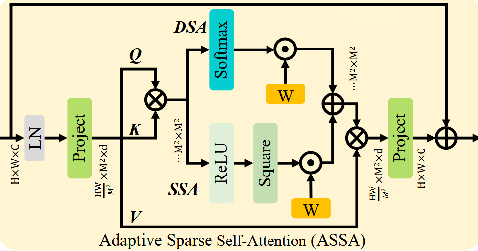
Fig 26. Adaptive Sparse Self-Attention (ASSA) [7]
Secondly, the AST replaces the standard MLP of the Transformer with what is known as a Feature Refinement Feed-forward Network (FRFN).
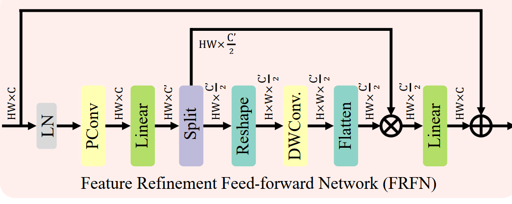
Fig 27. Feature Refinement Feed-forward Network (FRFN) [7]
Aside from being a post-attention network with convolutions that takes advantage of the spatial relationship of the tokens, the FRFN aims to address redundancy in the channel dimension after using ASSA. It utilizes partial convolutions, which only convolves on a portion of the channels, and depthwise convolutions, which convolves each channel independently, along with splitting the image along its channels and then combining the two halves to efficiently provide a post-ASSA transformation that can further attenuate the information from features extracted by the self-attention while giving the model some flexilibity to clear uninformative channels.
Putting it Together
Recall the structure of the Hybrid Attention Transformer (HAT):
Fig 28. HAT Architecture Overview [1].
One can see that the OCAB at the end of each RHAG acts as a sort of “gate” between RHAG blocks. Additionally, given the large key and value windows for the OCA, part of the purpose of the OCAB is to give each segment of the image a chance to incorporate together information from a larger portion of the image. However, it is likely that portions of these larger windows are not useful for the image reconstruction task, so this larger window allows for ample noise to seep through into our image tokens. So, we propose a modification to the HAT architecture that replaces the attention mechanism of the OCA with the Adaptive Sparse Attention scheme of the AST, and, subsequently, replaces the MLP of the OCAB with the FRFN. We hypothesize that this can temper the OCA and prevent noise issues from the larger windows, but can also act as a overall information gate for each window itself at the end of the RHAG, as the windows will perform cross-attention where the set of key and value pixel tokens are a superset of the query pixel tokens. Given that the principal design goal of the HAT is to use as much of the image as possible during reconstruction, the sparse attention may work well to balance that image-overuse, resulting in a model that has access to a large portion of the image but which can easily select which portions of the image are most useful.
Since we are giving the model this selective capability, we can likely afford to increase the size of the OCA window; in [1], they had found that an overlap ratio of 0.5 was optimal (meaning that key and value windows were 1.5x as large as the query window in each dimension), but a value of 0.75 produced slightly worse results. So, we propose that increasing the overlap ratio to 0.75 will better utilize the sparse attention, giving the model access to more information that it can select from, while remaining computationally efficient during the windowed cross-attention.
Specifically, in our experiment, we will be modifying the architecture of the HAT-S, the smallest HAT model, for practical reasons, and training it for doing 4x image upscaling.
Results
Here is a comparison of average PSNR on benchmark datasets between the base HAT-S and our model:
| |Set5 [8]| | |Set14 [9]| | |BSD100 [10]| | |Urban100 [11]| | |Manga109 [12]| | |
|---|---|---|---|---|---|
| HAT-S (baseline) | 32.92 | 29.15 | 27.97 | 27.87 | 32.35 |
| HAT-S + AST | 32.46 | 28.86 | 27.74 | 26.71 | 31.21 |
Unfortunately, our modification to the HAT-S was unable to match the results of the regular HAT-S. A possible reason is that the sparse attention is not particularly useful for 4x upscaling; there are few pixels in the starting image compared to the output image, so each one is more likely to hold important information than if we were doing something like 2x upscaling. Additionally, the size of the overlap window may be an issue: we did not get the chance to experiment with other sizes, so it is possible that the smaller 0.5 ratio may have actually worked better for our model, still benefitting from the sparse attention mechanism.
Here are a few samples from our validation sets:
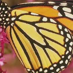
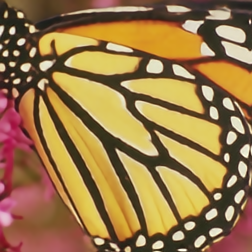
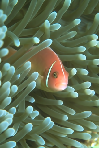
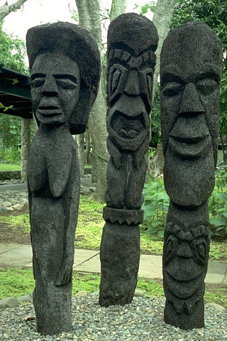
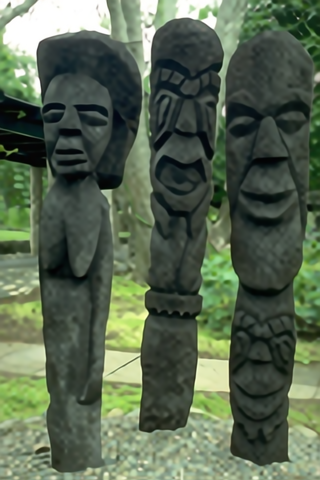
| HR Image | 4x Bicubic | HAT-S [1] | HAT-S + AST |
|---|---|---|---|
 |
 |
 |
 |
 |
 |
 |
 |
 |
 |
 |
 |
 |
 |
 |
 |
Fig 30. Comparison of HAT-S and our modification for images from Set5 [8], Set14 [9], and BSD100 [10].
We see similar qualitative peformance between HAT-S and our modification, though a closer inspection does confirm that our model produces slightly blurrier results.
In any case, the sparse attention mechanism and FRFN are interesting modifications to the Transformer; while our own experiment with the modification did not produce favorable results, we hope that future research continues to try to improve the current architectures and create entirely new ones.
Our Colab training script for the experiment can be found here, with supporting codebases here and here.
Conclusion
Image super-resolution (or, simply, image upscaling and reconstruction) is a foundational vision problem that has, in a sense, been around for as long as images have been on computers. In recent years, methods that use deep learning for computer vision have shown success for this problem, having the capacity to model very complex relationships between regions of an image to perform upscaling and de-degradation. However, this class of methods is not a monolith; there are many ways to utilize deep learning for this task, all with their own quirks, advantages, and disadvantages. The Hybrid Attention Transformer is an example of a Transformer-based method, and as such, it enjoys the capacity to scale very large to model complex reconstruction algorithms, but may suffer from issues of computational efficicency due to this scale; it stands out among other Transformer-based methods for its ability to create a very large receptive field for reconstruction, fully utilizing a given image for the task instead of just a segment of it. Look-Up Table methods sit on the other end of the computational complexity spectrum, doing away with an inference-time network and instead utilizing a quantized representation of deep network via a LUT. Of course, while this is very practically efficient, the method somewhat lacks in reconstruction accuracy and requires a fixed scale; developing extensions to the LUT to ameliorate these issues while mainitaining its speed is an active area of research. Finally, Unfolding Networks take an interesting, more fine-grained approach to the process of upscaling and de-degredation, by separating the problem into two distinct parts and leveraging learning-free, model-based methods in combination with learning-based methods to create an algorithm that is lightweight and robust. Based on the variety among existing super resolution architectures, it will be exciting to see what else is developed in the future.
In our experiment, we attempted to combine two existing super-resolution architectures, the Hybrid Attention Transformer and Adaptive Sparse Transformer, to determine if their opposing design philosophies could temper each other and result in a net-benefit. Unfortunately, this did not seem to be the case, as our modification to the HAT only worsened its performance. However, both of these architectures have been successful in their own right, and there likely exist yet-undiscovered modifications that will make them even more effective.
References
[1] X. Chen, X. Wang, J. Zhou, Y. Qiao and C. Dong, “Activating More Pixels in Image Super-Resolution Transformer,” 2023 IEEE/CVF Conference on Computer Vision and Pattern Recognition (CVPR), Vancouver, BC, Canada, 2023, pp. 22367-22377, doi: 10.1109/CVPR52729.2023.02142.
[2] Zhang, Kai, et al. “Deep Unfolding Network for Image Super-Resolution.” Proceedings of the IEEE/CVF Conference on Computer Vision and Pattern Recognition (CVPR), 2020, pp. 3217–3226.
[3] Jo, Younghyun, and Seon Joo Kim. “Practical Single-Image Super-Resolution Using Look-Up Table.” Proceedings of the IEEE/CVF Conference on Computer Vision and Pattern Recognition (CVPR), 2021, pp. 691–700. doi:10.1109/CVPR46437.2021.00075.
[4] N. Zhao, Q. Wei, A. Basarab, N. Dobigeon, D. Kouamé and J. -Y. Tourneret, “Fast Single Image Super-Resolution Using a New Analytical Solution for ℓ2 – ℓ2 Problems,” in IEEE Transactions on Image Processing, vol. 25, no. 8, pp. 3683-3697, Aug. 2016
[5] Park, S., Lee, S., Jin, K., & Jung, S.W. (2025). IM-LUT: Interpolation Mixing Look-Up Tables for Image Super-Resolution. In Proceedings of the IEEE/CVF International Conference on Computer Vision (ICCV) (pp. 14317-14325).
[6] Olaf Ronneberger, Philipp Fischer, and Thomas Brox. Unet: Convolutional networks for biomedical image segmentation. In International Conference on Medical image computing and computer-assisted intervention, pages 234–241. Springer, 2015.
[7] S. Zhou, D. Chen, J. Pan, J. Shi and J. Yang, “Adapt or Perish: Adaptive Sparse Transformer with Attentive Feature Refinement for Image Restoration,” 2024 IEEE/CVF Conference on Computer Vision and Pattern Recognition (CVPR), Seattle, WA, USA, 2024, pp. 2952-2963, doi: 10.1109/CVPR52733.2024.00285.
[8] M. Bevilacqua, A. Roumy, C. Guillemot, and M.-L. A. Morel, “Low-complexity single-image super-resolution based on nonnegative neighbor embedding,” in Br. Mach. Vis. Conf. (BMVC), 2012.
[9] R. Zeyde, M. Elad, and M. Protter, “On single image scale-up using sparse-representations,” in Int. Conf. Curves Surfaces, 2010, pp. 711–730.
[10] D. Martin, C. Fowlkes, D. Tal, and J. Malik, “A database of human segmented natural images and its application to evaluating segmentation algorithms and measuring ecological statistics,” in Proc. IEEE Int. Conf. Comput. Vis. (ICCV), vol. 2, 2001, pp. 416–423.
[11] J.-B. Huang, A. Singh, and N. Ahuja, “Single image super-resolution from transformed self-exemplars,” in Proc. IEEE Conf. Comput. Vis. Pattern Recognit. (CVPR), 2015, pp. 5197–5206.
[12] Y. Matsui, K. Ito, Y. Aramaki, A. Fujimoto, T. Ogawa, T. Yamasaki, and K. Aizawa, “Sketch-based manga retrieval using manga109 dataset,” Multimedia Tools Appl., vol. 76, no. 20, pp. 21 811–21 838, 2017.