Facial Emotion Recognition
This post details the current landscape of the Facial Emotion Recognition (FER) field. We discuss why this field is important and the current challenges it faces. We then discuss two datasets and two deep learning models for FER, one building off of ResNet and another extending ConvNeXt. Finally, we compare the two approaches and summarize our view on the research area.
Table of contents
1. Introduction
Facial Emotion Recognition (FER) is the task of identifying a person’s emotional state from an image or video of their face. Typical FER systems classify facial expressions into a fixed set of categories. With recent advances in deep learning and computer vision, FER has become an important research problem due to both its technical challenges and practical relevance.
Understanding emotion plays a key role in human communication, and enabling machines to recognize emotional cues is essential for advancing human-computer interaction. Facial expressions provide a direct and informative signal of emotion, making FER a valuable component in building human-aware artificial intelligence systems. As these systems improve, they will be able to respond more effectively to users by adapting their behavior based on emotional feedback. Some practical use cases are mental health monitoring, education technology, customer experience, and driver attention systems.
Despite this progress, FER remains a challenging task. Facial expressions can be subtle, ambiguous, and subjective, and are influenced by factors such as lighting, head pose, occlusion, and individual differences in facial structure. Emotions are also not always clearly separable and may overlap between categories, further complicating classification. This paper aims to explore recent advances and state-of-the-art models that address these challenges in facial emotion recognition.
2. Dataset
2.1. FER-2013
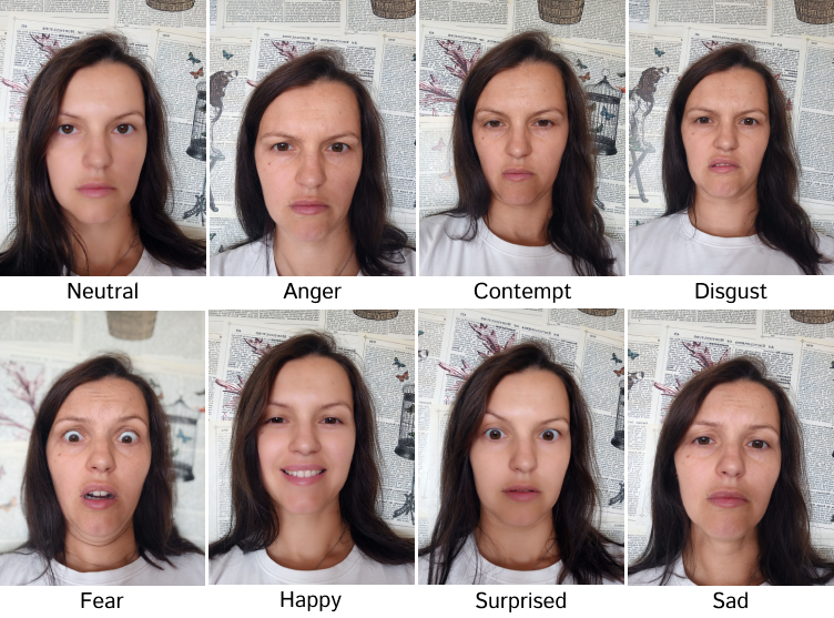
FER-2013 was the first large scale dataset for facial expression recognition. It was released on Kaggle in 2013 by Pierre Luc Carrier and Aaron Courville, and contains 35,887 48x48 grayscale images, with 32,298 released publicly for training/validation, and 3,589 hidden for testing. It divides images into seven categories: anger, disgust, fear, happiness, sadness, surprise, and neutral, though a human would recognize some images containing more subtle emotions (pride, embarrassment, contempt). This dataset is particularly challenging because it contains variations in lighting, background, and facial position.
The dataset was generated by using the Google Image Search API to search for facial images. Queries were constructed by combining emotion related keywords like “blissful”, “enraged”, and words related to gender, age, and ethnicity. In total, there were almost 600 query strings, and the first 1000 images returned from each query were kept. Then, the images were cropped using OpenCV facial recognition, and crowdsourced human labelers rejected incorrectly labeled images, modified crops if necessary, and filtered out duplicate images. Finally, the images were resized to 48x48 pixels and converted to grayscale.
However, the quality of labels and crops were underwhelming, likely due to crowd-sourced workers being paid little and prioritizing getting work done over ensuring tagging quality. One of the creators behind FER-2013 found human accuracy on a subset of the dataset to be only 65 ± 5%.
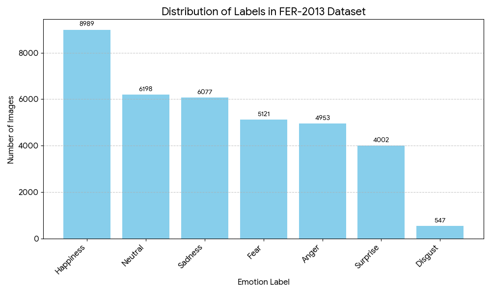
Additionally, there is a significant imbalance between classes, particularly toward emotions that are easier to recognize. The distribution of labels is shown below.
2.2. FER+ (2016)
To address these shortcomings, a group of researchers from Microsoft Research conducted a re-tagging of the FER-2013 dataset. They commissioned 10 taggers to label each image, obtaining a probability distribution of the emotion exhibited by each facial image (this is useful for one of the models discussed later). Additionally, the researchers introduced contempt as a new class. Some examples of corrected labels from the original FER dataset are shown below. The top labels are from FER, and the bottom labels are from FER+.
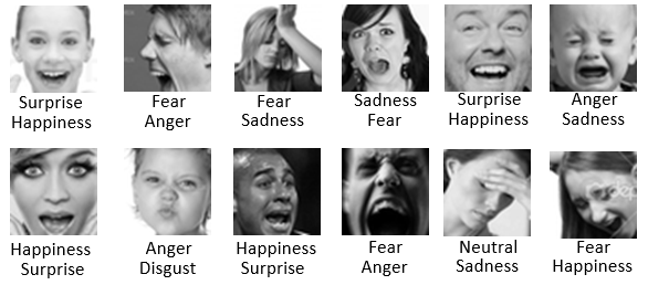
Some corrected image labels from FER+ [1].
177 images not containing faces or occluded faces were also removed.
However, one notable problem in the FER-2013 dataset that is still left unresolved by FER+ is the imbalance between classes. The distribution of labels from FER+ is shown below.
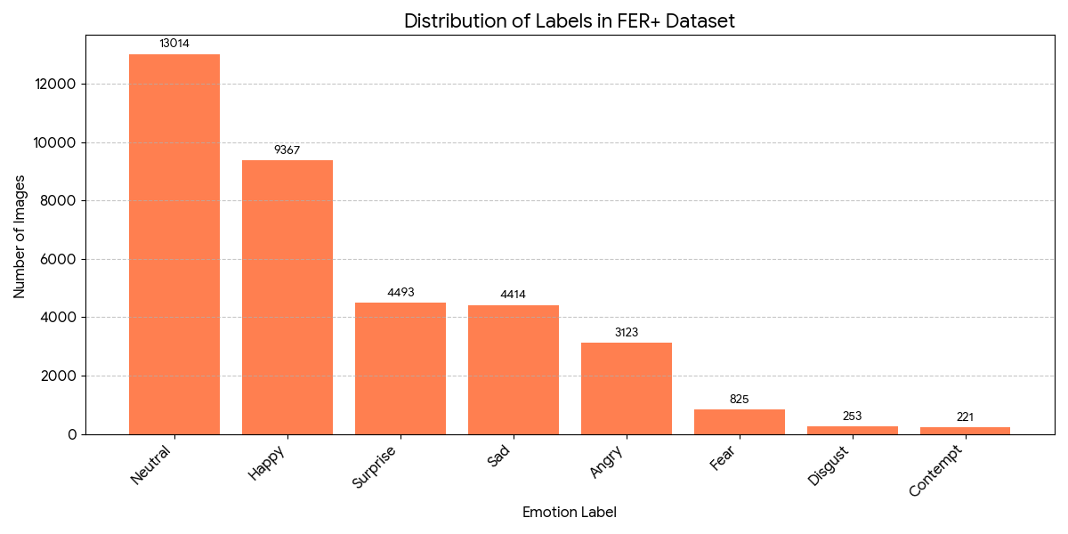
As you can see, there is a dramatic shift in the label distribution. For example, there were 5,121 images labeled as “fear” in the original FER, but only 825 in FER+.
3. ResFace
3.1. Overview
Facial Expression Recognition (FER) in real-world images is difficult because facial signals are subtle, easily hidden, and often influenced by pose variations. Traditional approaches train models to predict a single emotion label, assuming that each facial image reflects only a single pure expression. However, psychological studies and modern FER research show that real expressions often combine multiple emotions with varying intensities. This makes the single-label models insufficient for capturing the ambiguity that happens in human expression.
ResFace is proposed to solve these issues by introducing Label Distribution Learning (LDL) to model emotion mixtures and combat the noise caused by subjective annotations. It uses three key ideas, as shown in the Figure below.
- Local Feature Extraction via a ResNet backbone to learn and extract local, low-level features from the image.
- Channel-Spatial Feature Aggregation to suppress redundant features caused by occlusion and background noise while highlighting semantically relevant cues.
- Compact Feature Aggregation for label distribution learning (LDL) so that the network predicts a probability distribution of emotions rather than a single class.
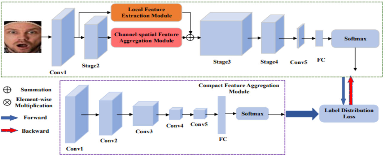
Overview of ResFace architecture [7].
3.2. Local Feature Extraction
The local feature extraction module is the first stage of the pipeline and is the backbone of ResFace. It uses ResNet-18 or ResNet-15 to capture the low-level and mid-level local features for FER. It is important to note that the design relies on the observation that local features are a basic necessity to classify emotional cues, as shown in prior research on FER. The figure below shows the full module and its ResNet-18 (or ResNet-50) backbone.
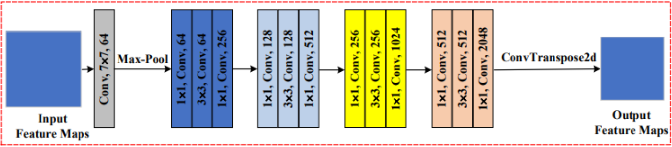
Architecture of Resnet-18 [7].
The input image of 224 x 224 x 3 is first passed through the standard Conv1 layer of Resnet, which is a 7 x 7 convolution followed by max-pooling. This produces an output feature map of size 56 x 56 x 64.
Then, the feature map is passed to subsequent residual blocks, where more complex local structures are captured through alternating 1 x 1 and 3 x 3 convolutional layers.This will contain spatially localized patterns like mouth curvature, eyebrow shape, and eye muscle tension, which carry the strongest emotional cues. Prior research on FER shows that these small-scale changes are important for distinguishing between expressions.
The colored blocks in the diagram visualize the progression through the ResNet stages. Unlike the standard ResNet architecture, ResFace also introduces a ConvTranspose2d upsampling layer at the end of the local extraction module. This operation is important because it prevents the network from collapsing local emotional detail too early, allowing the future modules to operate on feature maps with interpretable spatial structure.
3.3. Channel-Spatial Feature Aggregation Module
The primary goal of this module is to address some of the challenges in FER such as occlusion and pose variations. It also addresses one of the drawbacks of the local feature extraction: not everything in the picture is useful, as some information is just background noise or redundant data. This module is designed to aggregate the representative features with the original local features and learn global-salience, which helps distinguish informative features from non-informative features.
Below is an image depicting where this module is located in the entire pipeline. The aggregation method is applied after Stage 2 of the ResNet backbone. As you can see from the “+” sign, it is aggregated via summation with the result from the local feature extraction module and passed into Stage 3 of the ResNet backbone to continue through the network.
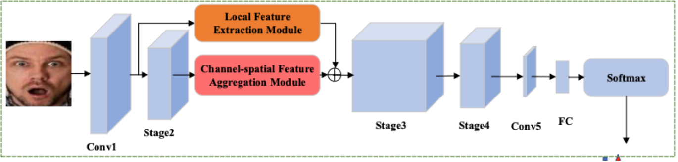
The Channel-Spatial Feature Aggregation Module’s position in the ResFace pipeline [7].
The module operates by calculating heatmaps that determine the importance of different features. The input to this module is high-level feature maps (denoted as Feastage2) which were generated by Stage 2 of the ResNet backbone.
The process is then split into 2 branches. The channel branch calculates the channel heatmaps (denoted as Zchannel). This consists of a Global Average Pooling layer followed by two Fully Connected layers. The spatial branch calculates the spatial heatmaps (denoted as Zspatial) which utilizes a series of convolutions, specifically a 1x1 followed by two 3x3s and finally a 1x1 layer to learn spatial features. The channel heatmap essentially tells us what type of information is important, while the spatial heatmap tells us where in the image the important information is located. Below is a diagram that shows these 2 branches:
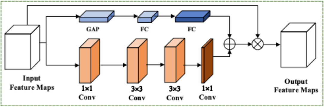
Channel-Spatial Feature Aggregation Module [7].
Next, the heatmaps of the 2 branches are combined. It is important to note that both heatmaps are resized to match dimensions prior to adding them together. A sigmoid function is applied to this sum for normalization, generating the final combined heatmap (denoted as Z(Feastage2)). This is denoted by the “+” sign in the diagram above. The mathematical formula is as below:
\[Z(Fea_{stage2})=\sigma(Z_{channel}(Fea_{stage2})+Z_{spatial}(Fea_{stage2}))\]Once the combined heatmap is generated, it is applied to the original image features through element-wise multiplication. This is denoted by the “x” sign in the diagram above. This effectively weighs the original features by their calculated importance with the formula below. It suppresses useless information and highlights important features, which allows the model to better handle challenges such as face rotation and occlusion.
\[Fea_{modulated}=(Fea_{stage2})\otimes Z(Fea_{stage2})\]Finally, circling back to the original pipeline, the final feature set (denoted as Feafinal) is calculated via addition of the local and modulated features. Thus, the model retains original local information while benefiting from this global focus. This is what is passed into Stage 3 of the ResNet backbone. The formula is as below:
\[Fea_{final}=Fea_{local} + Fea_{modulated}\]3.4. Compact Feature Aggregation Module & Label Distribution Learning (LDL)
The Compact Feature Aggregation Module, as shown below, is the final processing stage in the ResFace pipeline before the system makes a classification decision. It is essential to note that this is not combined with the main architecture of the Local Feature Extraction Module + Channel-Spatial Feature Extraction Module, but rather done in parallel in order to compute the LDL loss at the end of the training process.
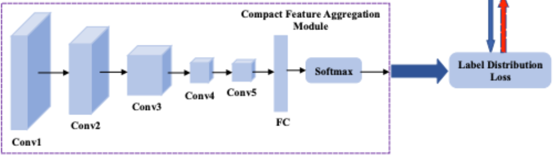
The Compact Feature Aggregation Module’s position in the ResFace pipeline [7].
Beginning with the output of Conv1, the feature maps are passed through four consecutive convolutional blocks (Conv2 → Conv3 → Conv4 → Conv5). Each block reduces the spatial redundancy and preserves the semantically meaningful information related to facial expression intensity. As described in the name, the stacked convolutions filter the representation into a compact embedding that emphasizes the global structural cues rather than the fine-grained local texture. This differs from the local feature extraction module because the compact aggregation makes a more abstract feature space that is better aligned with the needs of distribution based supervision.
After the convolutional stack, the resulting feature map is flattened and passed to a fully connected layer. This output is then passed through a softmax function that produces a feature vector \(F_v = (F_{v_0}, F_{v_1}, F_{v_2}, ... , F_{v_{l−1}})\). This is the learned label distribution, which will then be used in label distribution learning.
Although traditional facial expression recognition models treat each image as belonging to exactly one emotion class, and as mentioned in the introduction, studies show that expressions often reflect mixtures of emotions with varying intensities. To address this, ResFace uses Label Distribution Learning (LDL), in which each image is supervised not by a single label but by a probability distribution over all emotion categories.
LDL is implemented using a Label Distribution Generator (LDG), which produces a soft target distribution \(Dis = (Dis_0,Dis_1,...,Dis_{l-1})\) where \(\sum^{l-1}_{j=0}\phi_j=1\).
The softmax output from the Compact Feature Aggregation Module is treated as the model’s predicted distribution \(Dis\). These two distributions are then compared during training, allowing ResFace to learn from mixed or ambiguous emotional cues rather than relying on a single hard label.
3.5. Train, Validation, Test Set-Up
This model has been validated on 2 primary datasets: RAF-DB and FER+. RAF-DB contains 12,271 training set images, 3,068 testing set images, with labels annotated with 7 basic emotion classes. FER+ contains 28,709 training set images, 3,859 validation set images, and 3,589 testing set images.
Before the images enter the network, they are preprocessed by resizing to 224 x 224 dimensions with random cropping and random horizontal flipping augmentation. This ensures consistency and prevents the model from overfitting by memorizing the training data.
ResFace deviates from typical models in the way that instead of training the model to predict a single emotion (eg. 100% sad, 100% happy), label distribution learning is used. The motivation behind this is the fact that real-world emotions are often a mix of different emotions. Therefore, the LDG is used to create a soft distribution of probabilities of labels rather than a single hard label. The loss function used here is Cross-Entropy loss. It measures the difference between the distribution predicted by ResFace and the distribution generated by the LDG. The specific formula is as below. N is the number of samples, l is the number of emotion categories, and dis represents the predicted label distribution.
\[Loss_{all}=-\frac{1}{N\times l}\sum^{N-1}{i=0}\sum^{l-1}_{m=0}dis^i_m\log(\overline{dis}^i_m)\]A typical technical configuration of this model is as follows. It uses a PyTorch framework running on NVIDIA Titan RTX. The ResFace architecture is initialized by training it from scratch. It uses Stochastic Gradient Descent (SGD) as its optimizer with an initial learning rate of 0.1 and batch size of 64.
3.6. Results
To evaluate the effectiveness of the ResFace model, experiments were conducted on two widely used facial expression recognition datasets: RAF-DB and FER+. The results demonstrate consistent improvements when integrating the three major components of ResFace:
- Local Feature Extraction
- Channel–Spatial Feature Aggregation
- Compact Feature Aggregation + Label Distribution Learning (LDL)
[7]
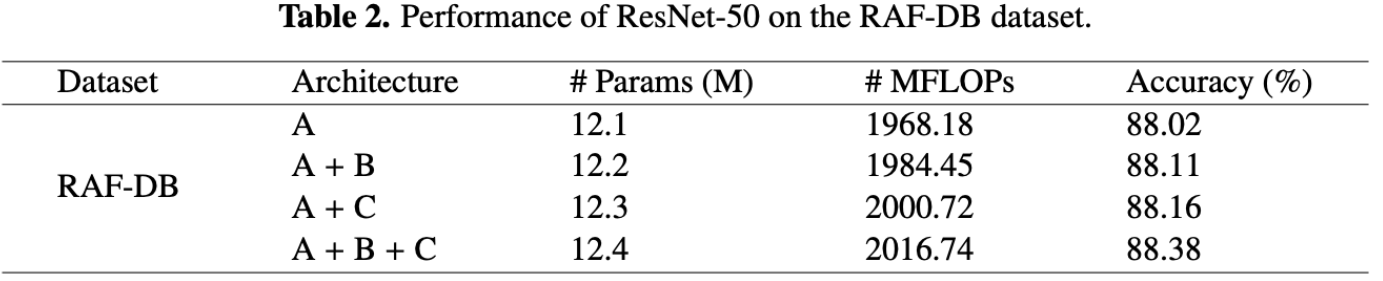
Table 2 displays the accuracy improvements in the RAF-DB dataset when using a ResNet-50 backbone. Starting from the baseline architecture (A), an accuracy of 88.02% is achieved. When the channel-spatial aggregation module is added (A + B), performance improves to 88.11%, indicating that attention over spatial locations and feature channels helps suppress redundant information. Adding the compact feature aggregation module with label distribution learning (A + C) further increases accuracy to 88.16%. The best performance is obtained when all components are combined (A + B + C), achieving an accuracy of 88.38%.
[7]
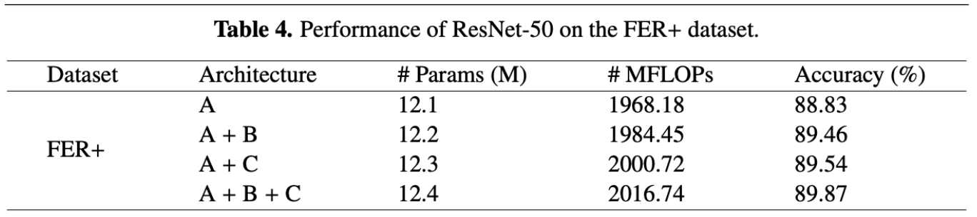
A similar trend is seen on the FER+ dataset using the same ResNet-50 backbone, as shown in table 4. The baseline ResNet-50 model (A) achieves an accuracy of 88.83%. Adding the channel–spatial aggregation module (A + B) improves accuracy to 89.46%, while adding the compact aggregation module with LDL (A + C) achieves 89.54%. When all components are integrated, the model reaches an accuracy of 89.87%, which is the highest among all tested configurations. Since FER+ contains many ambiguous and mixed expressions, the performance gain underscores the effectiveness of label distribution learning in capturing nuanced emotional information.
[7]
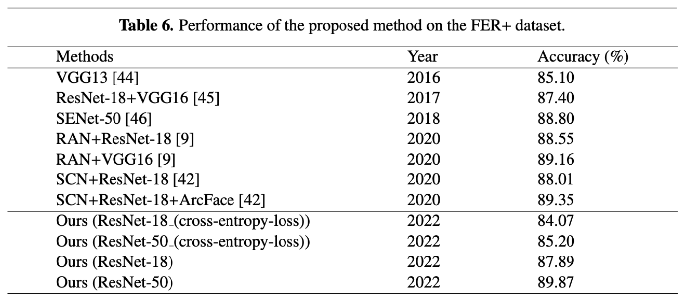
[7]
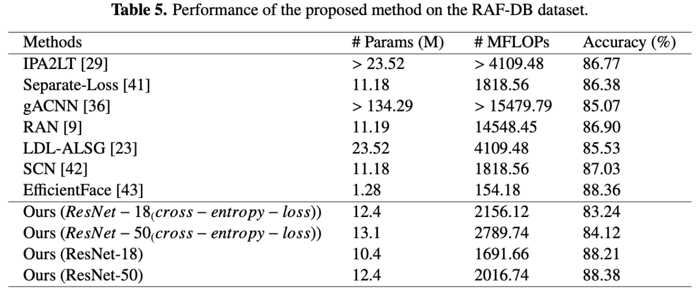
Tables 5 and 6 compare ResFace with several state-of-the-art FER methods on RAF-DB and FER+, respectively. On RAF-DB, ResFace achieves accuracies of 88.21% with ResNet-18 and 88.38% with ResNet-50, outperforming many existing approaches, including RAN, LDL-ALSG, SCN, and IPA2LT. Despite having a relatively small number of parameters, ResFace achieves competitive performance compared to more complex models like gACNN, which requires higher computational cost. The results show that ResFace achieves a good balance between accuracy and efficiency.
On FER+, ResFace achieves an accuracy of 87.89% with ResNet-18 and 89.87% with ResNet-50, as shown in Table 6. The ResNet-50 version achieves the highest accuracy among the compared methods, surpassing traditional CNN-based approaches and matching or beating more recent attention-based models. Overall, the experimental results show that combining local feature learning, attention-based aggregation, and label distribution learning enables ResFace to model emotional ambiguity effectively while maintaining computational efficiency.
3.7. Tradeoffs
The most significant advantage of this model is its use of Label Distribution Learning instead of single-label classification. This addresses the real world emotional complexity and reduces noise. Similarly, the model utilizes a “parallel” architecture during the training phase, specifically a Label Distribution Generator (LDG), to compute the loss, rather than relying solely on static hard labels. During the training stage, the LDG is fixed, acting as a stable teacher that guides the main architecture to learn informative features without the instability of optimizing the generator simultaneously. Finally, the core of the model, the Channel-Spatial Feature Aggregation Module improves feature quality by combining local feature importance with global salience. This solves the real-world problem of occlusion and pose variance.
With this, comes the difficulty of increased computational complexity and parameter count. The complexity of calculation increases as well, as the number of floating point operations is also higher. On the other hand, this increase could be justified by higher accuracy.
4. EmoNeXt
4.1. Overview
Classical Facial Emotion Recognition (FER) approaches typically follow a two-step process: first, manually defining and extracting facial features (geometric or appearance-based), and second, classifying those features using models like Support Vector Machines (SVM) or MultiLayer Perceptrons (MLP).
The fundamental problem with this conventional methodology is that these two steps are performed separately, which can result in poorer performance, in particular when the dataset contains numerous sources of variability. This issue is addressed by DNNs which learn discriminative feature representations and simultaneously determine classification parameters directly from raw data.
The EmoNeXt framework was specifically developed to build upon the latest convolutional models (specifically ConvNeXt) and solve the problem of achieving high accuracy in complex, variable FER datasets. It addresses critical recognition challenges by integrating modules that automatically handle spatial transformations (like scale and rotation) and enhance the network’s ability to discriminate between features, aiming to significantly improve upon the original ConvNeXt network and existing state-of-the-art models.
EmoNeXt’s architecture builds off of ConvNeXt, integrating several specialized components to enhance robustness, feature extraction, and generalization capabilities for FER.
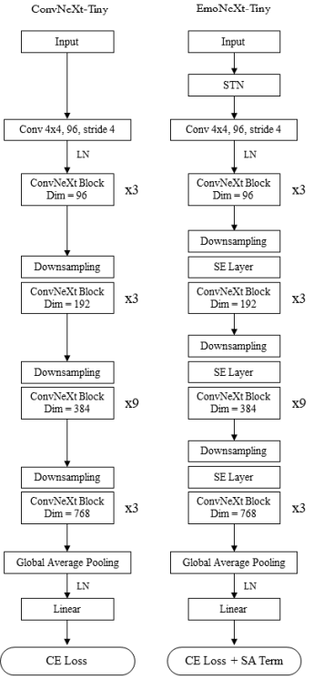
EmoNeXt architecture [2].
The first specialized component is the Spatial Transformer Network (STN). This is a differentiable geometric transformation module that enables the network to automatically learn and apply spatial transformations to input images. This component is particularly valuable for FER because it allows the model to handle performance-degrading variations such as changes in scale, rotation, and translation of the facial image.
Following the STN, the inputs are passed through the ConvNeXt’s patchify module. This module efficiently down-samples the input image and captures relevant initial features using a non-overlapping convolution with a 4 x 4 kernel size.
The downscaled inputs proceed through the main ConvNeXt stages. A key modification in EmoNeXt is that each stage is immediately followed by a Squeeze-and-Excitation (SE) block. SE blocks enhance the model’s representational power by adaptively recalibrating channel-wise features. They operate by emphasizing informative channels and suppressing less relevant ones, which improves the extraction of discriminative facial features for accurate emotion classification.
To optimize the model’s performance and improve generalization, EmoNeXt utilizes a final loss function (\(L_{final}\)) that combines the standard Cross-Entropy Loss (\(L_{CE}\)) with a Self-Attention (SA) regularization term (\(L_{SA}\)). The SA regularization term minimizes the variance of the attention weights, bringing the weights to be closer to their mean value (\(\overline{W}\)). This process promotes balanced importance across generated features, thereby helping the model produce more compact feature vectors during training.
4.2. Spatial Transformer Network
To account for variance in scale, rotation, skew, and translation between facial images, the authors introduced a Spatial Transformer Network as the first layer of the Network. Spatial Transformer networks learn an affine transformation (a transformation that preserves lines) to sample a specific region of it, as if cropping the image into a parallelogram.
![]()
Spatial Transformer Network modules [2].
The Spatial Transformation Network consists of three parts: a localization network, which computes the transformation, a sampling grid generator, which creates a set of points where the input map should be sampled to produce the transformed output, and a sampler, which takes the sampling grid and the input image to produce the output map.
The localization network is essentially a CNN whose final fully connected layer has an output size of 6, one for each value of the 2 x 3 affine transformation matrix. The full architecture is shown below. Since the transformation is generated by a neural network, this means that the transformation is (1) different for each input image and (2) learned during training. Note that the affine transformation is from the output space to the input space, which simplifies sampling.
| Layer Type | Input Size | Parameters | Output Size |
|---|---|---|---|
| Input Image | 3×224×224 | - | 3×224×224 |
| Conv2d | 3×224×224 | C: 3→8, K=7 | 8×218×218 |
| BatchNorm2d | 8×218×218 | - | 8×218×218 |
| MaxPool2d | 8×218×218 | K=2,S=2 | 8×109×109 |
| ReLU | 8×109×109 | - | 8×109×109 |
| Conv2d | 8×109×109 | C: 8→10, K=5 | 10×105×105 |
| BatchNorm2d | 10×105×105 | - | 10×105×105 |
| MaxPool2d | 10×105×105 | K=2,S=2 | 10×52×52 |
| ReLU | 10×52×52 | - | 10×52×52 |
| Flatten | 10×52×52 | - | 27040 units |
| Linear | 27040 units | - | 32 units |
| ReLU | 32 units | - | 32 units |
| Linear (Output) | 32 units | - | 6 units |
The grid generator applies the affine transformation above to each pixel in the output to generate a grid of points in the image to sample from. This grid is represented as a tensor of shape \((N, H_{out}, W_{out}, 2)\), where N represents the batch size, and the 2 corresponds to an (x, y) coordinate pair. These coordinates are normalized to the range \([-1, 1]\) where \((-1, -1)\) is the top-left corner, \((1, 1)\) is the bottom-right corner, and \((0, 0)\) is the center of the image. This normalization makes the transformation scale-invariant to the actual pixel dimensions of the input.
For every \((x,y)\) coordinate in the grid, the sampler uses bilinear interpolation to fill in a value for each pixel in the output. Note that bilinear interpolation is fully differentiable, allowing for the entire Spatial Transformation Network to be updated through backpropagation.
4.3. ConvNeXt
The architecture known as ConvNeXt was introduced in 2022 as a pure convolutional model. Its development was largely inspired by recent advancements in Vision Transformers, but ConvNeXt was specifically designed to compete effectively with these state-of-the-art models while maintaining the fundamental simplicity and efficiency of Convolutional Neural Networks (CNNs).
ConvNeXt incorporates several enhancements adapted from modern architectures and builds upon the design of a standard ResNet. These modifications define the efficiency and performance of the core ConvNeXt block.
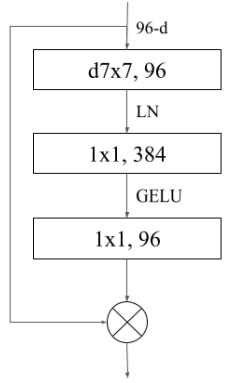
ConvNeXt block [2].
One modification the ConvNeXt block utilizes is larger kernel-sized and depthwise convolutions. It employs an inverted bottleneck design, which is critical for enhancing performance while simultaneously lowering the overall floating-point operations (FLOPs) of the network. This design helps increase the network width in an efficient manner.
ConvNeXt also adapted normalization and activation techniques often seen in advanced Transformer models to achieve slightly better performance. Specifically, it replaced the traditional ReLU activation function with GELU (Gaussian Error Linear Units) and substituted Batch Normalization (BN) with Layer Normalization (LN) as the normalization technique.
Scalability was also a significant focus for this model. The architecture is flexible and was developed in multiple versions (Tiny, Small, Base, Large, and XLarge). These versions are differentiated by varying the number of channels (C) and blocks (B) used within each stage.
Lastly, when utilized in downstream tasks, such as in the EmoNeXt framework, the ConvNeXt architecture can leverage the pretrained weights sourced from the large-scale ImageNet-22k dataset. To ensure compatibility with these weights, input images must typically be resized.
4.4. Squeeze and Excitation Blocks
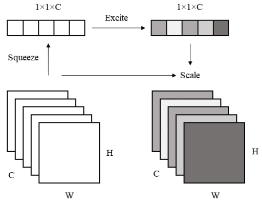
Squeeze and Excitation Block module [2].
The Squeeze and Excitation allows the network to give different weights to each channel, almost as if applying channel-wise attention.
In the Squeeze phase, global average pooling is applied to each channel of the input feature map, which results in a (1, 1, C) tensor. In the excite phase, this tensor is transformed using two fully connected layers. The first linear layer reduces the tensor to (1, 1, C/r) and is followed by a ReLU, and the second linear layer takes the tensor back to (1, 1, C) and is followed by a Sigmoid. The authors chose r=16. This bottleneck structure makes the computation more efficient and promotes learning important features over noise. The resulting attention weights are then multiplied element-wise with the original feature map, emphasizing important channels and suppressing less relevant ones.
4.5. Training
For training, a pretrained ConvNeXt on the ImageNet-22k dataset was modified to fit the architecture described above, and was fine tuned using the FER-2013 dataset discussed in an earlier section. To reiterate, the dataset contains 35,887 grayscale images. 28,709 are used for training, 3,589 are used for validation, and 3,589 are used for testing. There are seven emotion categories: anger, disgust, fear, happiness, sadness, surprise, and neutral, though the number of samples varies significantly between classes. Even though the images from FER-2013 are 48x48, they are resized to 224x224 to fit the expected input size of ConvNeXt.
For training, the AdamW optimizer with a learning rate of 1e-4 was used in conjunction with a cosine delay schedule. Random crops and random rotation were applied to the training data. Stochastic depth (randomly removing residual blocks) and label smoothing (adding noise to ground truth label) were used for regularization. Weights are updated using an exponential moving average technique, which reduces overfitting by smoothing out weight updates.
Additionally, the authors employed Mixed Precision Training, which uses both 16-bit and 32-bit floating point numbers, thus reducing memory consumption and accelerating training. The model weights and optimizer state are stored using 32 bits, but the technique attempts to use 16-bit floating points when possible, such as during the forward pass and gradient calculations. Note that loss scaling is required, where gradients are multiplied by a large factor before backpropagation to prevent small gradients from underflowing in the FP16 format. The gradients are later scaled back down before updating the FP32 master weights.
All five sizes (T, S, B, L, and XL) of both ConvNeXt and EmoNeXt were trained using an Nvidia T4 GPU (16GB VRAM).
4.7. Code Implementation
Architecture - Squeeze-and-Excitation (SE) Block
class SELayer(nn.Module):
    def __init__(self, channel, reduction=16):
        super(SELayer, self).__init__()
        self.avg_pool = nn.AdaptiveAvgPool2d(1)
        self.fc = nn.Sequential(
            nn.Linear(channel, channel // reduction, bias=False),
            nn.ReLU(inplace=True),
            nn.Linear(channel // reduction, channel, bias=False),
            nn.Sigmoid(),
        )
    def forward(self, x):
        b, c, _, _ = x.size()
        y = self.avg_pool(x).view(b, c)
        y = self.fc(y).view(b, c, 1, 1)
        return x * y.expand_as(x)
Architecture - Dot Product Self-Attention Mechanism
class DotProductSelfAttention(nn.Module):
    def __init__(self, input_dim):
        super(DotProductSelfAttention, self).__init__()
        self.input_dim = input_dim
        self.norm = nn.LayerNorm(input_dim)
        self.query = nn.Linear(input_dim, input_dim)
        self.key = nn.Linear(input_dim, input_dim)
        self.value = nn.Linear(input_dim, input_dim)

    def forward(self, x):
        # ... calculation of query, key, value ...
        scores = torch.matmul(query, key.transpose(-2, -1)) * scale
        attention_weights = torch.softmax(scores, dim=-1)
        attended_values = torch.matmul(attention_weights, value)
        output = attended_values + x
        return output, attention_weights
This module outputs attention_weights, which is critical for calculating the SA regularization loss.
EmoNeXt Class - STN Initialization
The STN is defined as two main components within the EmoNeXt class initialization: the localization network (composed of standard convolutional layers and pooling) and the fc_loc regressor, which calculates the affine transformation matrix.
class EmoNeXt(nn.Module):
    def __init__(
        self,
        # ... other parameters ...
    ):
        # ...
        # Spatial transformer localization-network
        self.localization = nn.Sequential(
            nn.Conv2d(3, 8, kernel_size=7),
            nn.BatchNorm2d(8),
            nn.MaxPool2d(2, stride=2),
            nn.ReLU(True),
            nn.Conv2d(8, 10, kernel_size=5),
            nn.BatchNorm2d(10),
            nn.MaxPool2d(2, stride=2),
            nn.ReLU(True),
        )
        # Regressor for the 3 * 2 affine matrix
        self.fc_loc = nn.Sequential(
            nn.Linear(10 * 52 * 52, 32), nn.ReLU(True), nn.Linear(32, 3 * 2)
        )
        # ...
EmoNeXt Class - STN Execution
The stn function applies the learned transformation. It takes the input, runs it through the localization and regressor networks to get the affine matrix (theta), and uses F.affine_grid and F.grid_sample to generate the transformed output image.
def stn(self, x):
    xs = self.localization(x)
    xs = xs.view(-1, 10 * 52 * 52)
    theta = self.fc_loc(xs)
    theta = theta.view(-1, 2, 3)
    grid = F.affine_grid(theta, x.size(), align_corners=True)
    x = F.grid_sample(x, grid, align_corners=True)
    return x
EmoNeXt Class - Integrating SE Blocks into ConvNeXt Stages
When defining the intermediate downsampling layers (which occur between the ConvNeXt stages), the SELayer is explicitly added after the convolution and normalization steps for stages 1, 2, and 3.
for i in range(3):
            downsample_layer = nn.Sequential(
                LayerNorm(dims[i], eps=1e-6, data_format="channels_first"),
                nn.Conv2d(dims[i], dims[i + 1], kernel_size=2, stride=2),
                SELayer(dims[i + 1]), # SE Block insertion point
            )
            self.downsample_layers.append(downsample_layer)
Loss Function with Self-Attention Regularization
Finally, the forward function of EmoNeXt demonstrates how the Self-Attention (SA) regularization term is calculated and added to the standard loss, promoting balanced attention weights and compact feature vectors.
def forward(self, x, labels=None):
    x = self.stn(x) # Apply STN first
    x = self.forward_features(x)
    _, weights = self.attention(x) # Get attention weights
    logits = self.head(x)

    if labels is not None:
        mean_attention_weight = torch.mean(weights)
        attention_loss = torch.mean((weights - mean_attention_weight) ** 2) # LSA calculation
        loss = F.cross_entropy(logits, labels, label_smoothing=0.2) + attention_loss # Lfinal = LCE + LSA
        return torch.argmax(logits, dim=1), logits, loss

    return torch.argmax(logits, dim=1), logits
The attention_loss is calculated as the mean squared difference between the individual attention weights and their overall mean. This loss is then added to the classification loss (Cross-Entropy Loss), weighted by an implicit lambda=1 in this code snippet, to finalize the training objective.
4.8. Results
[2]
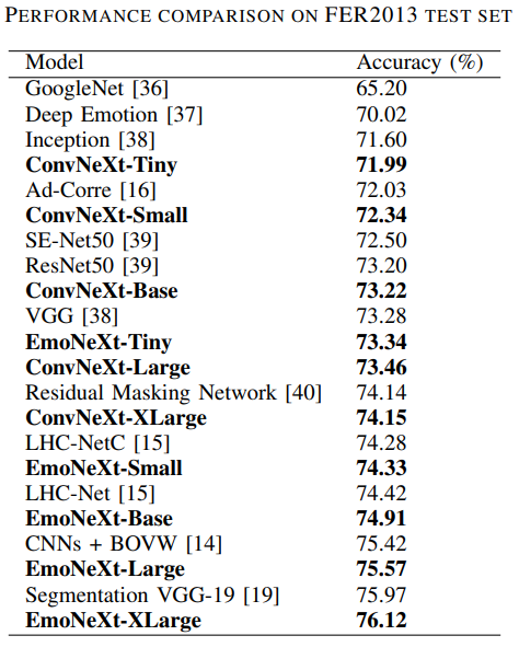
The EmoNeXt models considerably outperform their ConvNeXt counterparts, and the EmoNeXt-XLarge model achieves state of the art accuracy on FER-2013. Predictably, accuracy increases with model size. However, EmoNeXt-Small is especially notable because it has a notable jump in performance with EmoNeXt-Tiny, while only slightly falling behind EmoNeXt-Base. It also surpasses Residual Masking Network and LHC-NetC, which are larger models.
4.9. Pros and Cons
The EmoNeXt framework, while complex, provides significant advantages for Facial Emotion Recognition (FER) compared to existing models, primarily due to its specialized architectural components.
A key strength is its classification accuracy, with the EmoNeXt-XLarge model achieving 76.12% accuracy on the FER2013 test set, a score that surpasses the current best state-of-the-art single network architecture, the Segmentation VGG-19 model (75.97%). Even the smaller EmoNeXt-Tiny and EmoNeXt-Small variants, achieving 73.34% and 74.33% accuracy, respectively, demonstrated superior performance compared to well-known models like ResNet50 and the original ConvNeXt counterparts.
Despite this great accuracy, EmoNeXt faces several limitations, largely tied to its data environment and size requirements for peak performance. For example, due to the highly unbalanced distribution of classes present in the FER2013 dataset, the model is heavily reliant on it for training and evaluation. Specifically the EmoNeXt-XLarge configuration is often necessary to reach high levels of accuracy.
Given that larger versions of ConvNeXt involve greater numbers of channels and blocks, these high-performing models likely entail substantial computational resource requirements. Additionally, the architecture is very complex, combining the ConvNeXt base with STN, SE blocks, and SA regularization. This intricacy makes the system much more complex than a standard convolutional network.
5. Comparison
5.1. Architecture
ResFace and EmoNeXt adopt fundamentally different architectural designs for facial emotion recognition. ResFace is built on a traditional ResNet backbone and adds modules that directly address known challenges in FER, such as emotional ambiguity, occlusion, and pose variation. Its design focuses on local feature extraction followed by attention-based channel-spatial aggregation, and it introduces a parallel compact feature aggregation branch that is dedicated to Label Distribution Learning (LDL). This design allows ResFace to model an emotion by predicting probability distributions rather than relying solely on a single hard class label. This makes it well-suited for datasets with subjective or ambiguous emotions.
In contrast, EmoNeXt is based on the ConvNeXt architecture, a modern convolutional model inspired by Vision Transformers. Rather than introducing an external teacher network like in ResFace, EmoNeXt integrates multiple feature-enhancing components directly into the backbone. These include a Spatial Transformer Network (STN), placed at the very beginning of the network to normalize geometric variations in facial images. It also includes Squeeze-and-Excitation (SE) blocks, which are inserted after every ConvNeXt stage to recalibrate channel-wise feature importance and to add a self-attention regularization term, encouraging compact and balanced feature representations during training. Unlike ResFace, EmoNeXt relies on standard single-label classification and does not explicitly model emotion ambiguity through label distributions. Instead, it emphasizes stronger feature learning through attention, normalization, and regularization within the backbone itself.
Overall, ResFace introduces complexity through parallel learning objectives and distribution-based supervision, while EmoNeXt increases complexity within the backbone by stacking multiple advanced modules on top of ConvNext.
5.2. Efficiency
From an efficiency perspective, ResFace is designed to achieve strong performance with relatively lightweight models. The authors demonstrate that even the ResNet-18 variant performs competitively, containing approximately 10.4 million parameters, while the ResNet-50 version remains compact at around 12.4 million parameters and around 2,000 MFLOPs. Although ResFace introduces additional modules such as the LDG during training, this teacher network is removed during inference, meaning it does not add overhead to the deployed model. As a result, ResFace has low computational cost while benefiting from label distribution learning.
EmoNeXt, on the other hand, tends to be more computationally demanding, specifically for its higher-performing variants. While smaller versions such as EmoNeXt-Tiny and EmoNeXt-Small already outperform several baseline models, the highest accuracy is achieved by EmoNeXt-Xlarge. This implies significantly higher computational and memory requirements compared to ResFace’s lightweight ResNet-based versions. EmoNeXt employs mixed precision training and exponential moving average (EMA) optimization techniques to reduce GPU memory usage and stabilize training. Even with these optimizations, EmoNeXt prioritizes representational power over efficiency, making it more resource-intensive than ResFace.
5.3. Performance
In terms of performance, both models achieve strong results within their respective evaluation settings. ResFace is evaluated on FER+ and RAF-DB, datasets that feature refined annotated labels. On FER+, ResFace achieves accuracies of 89.87% with ResNet-50 and 87.89% with the lightweight ResNet-18 variant, demonstrating both high accuracy and efficiency. On RAF-DB, the ResNet-50 version reaches 88.38%, outperforming many existing FER approaches while maintaining efficiency.
EmoNeXt is evaluated on the original FER2013 dataset, which is known for noisy annotations and class imbalance. Under these more challenging conditions, EmoNeXt-XLarge achieves 76.12% accuracy, surpassing the previous state-of-the-art Segmentation VGG-19 model. Even the EmoNeXt-Tiny variant achieves 73.34%, outperforming standard CNN-based methods on the same dataset. While EmoNeXt’s raw accuracy scores are lower than those achieved by ResFace, this difference highly reflects dataset difficulty rather than model capability.
In summary, ResFace excels in scenarios with prevalent emotional ambiguity and mixed expressions, leveraging label distribution learning to model these states. EmoNeXt, by contrast, demonstrates strong utility for misalignment, rotation, and scale variation through spatial transformations and backbone-level attention mechanisms. Both models represent state-of-the-art solutions, optimized for different challenges within facial expression recognition.
6. Conclusion
The objective of this technical report was to analyze modern Deep Learning (DL) approaches designed to improve Facial Emotion Recognition (FER), a task considered fundamental to effective social interactions and necessary for applications across fields like healthcare and human-computer interaction. We primarily focused on methods evaluated using the FER2013 dataset, which serves as a widely recognized but inherently challenging benchmark due to its size, poor label quality, and significant class imbalance. Specifically, we detailed the motivation, architecture, and performance of two contemporary frameworks: ResFace and EmoNeXt. ResFace addressed the subjective and ambiguous nature of real-world expressions by employing Label Distribution Learning (LDL), which supervises the network using a probability distribution over emotion categories rather than a single hard label. Conversely, the EmoNeXt framework, built on an adapted ConvNeXt architecture, focused on achieving state-of-the-art accuracy by integrating specialized modules like the Spatial Transformer Network (STN) to automatically handle spatial variations, and Squeeze-and-Excitation (SE) blocks for adaptive channel-wise feature recalibration.
The most difficult challenge identified across modern FER research is fundamentally tied to data quality and distribution. Foundational datasets like FER2013 are plagued by defects, including misclassified images and highly unbalanced distributions across emotion categories, which dramatically impede a model’s ability to generalize effectively. Furthermore, achieving the highest performance levels necessitates increasingly complex DL models, such as the EmoNeXt-XLarge or EfficientNetB7 configurations. These large-scale models place severe demands on computational resources, often leading to limitations in GPU memory and maximum continuous execution time during the training process. Beyond data quality, models must also robustly extract discriminative features from faces despite real-world noise sources like pose variations, partial occlusion, and variations in scale.
Based on the demonstrated performance of complex architectures and the critical role of data preparation, we predict that the best future models will emerge from combining enhanced, diverse datasets with the next generation of powerful feature extractors. While EmoNeXt showed that advanced CNNs can compete with state-of-the-art Vision Transformers, the continued exploration of pure Transformer or hybrid models combined with vastly superior, defect-free datasets would maximize the architecture’s ability to capture the subtle, fine-grained emotional feature embeddings needed to truly master complex FER tasks.
7. References
[1] Barsoum, E., Zhang, C., Canton Ferrer, C., & Zhang, Z. (2016). Training Deep Networks for Facial Expression Recognition with Crowd-Sourced Label Distribution. ACM International Conference on Multimodal Interaction (ICMI).
[2] El Boudouri, Y., & Bohi, A. (2023). EmoNeXt: an Adapted ConvNeXt for Facial Emotion Recognition. In 2023 IEEE 25th International Workshop on Multimedia Signal Processing (MMSP) (pp. 1–6). IEEE. https://doi.org/10.1109/MMSP59012.2023.10337732
[3] Goodfellow, I. J., Erhan, D., Carrier, P. L., Courville, A., Mirza, M., Hamner, B., Cukierski, W., Tang, Y., Thaler, D., Lee, D.-H., et al. (2013). Challenges in representation learning: A report on three machine learning contests. Neural information processing (pp. 117–124). Springer.
[4] Hu, J., Shen, L., & Sun, G. (2017). Squeeze-and-Excitation Networks. CoRR, abs/1709.01507. Retrieved from http://arxiv.org/abs/1709.01507
[5] Jaderberg, M., Simonyan, K., Zisserman, A., & Kavukcuoglu, K. (2015). Spatial Transformer Networks. CoRR, abs/1506.02025. Retrieved from http://arxiv.org/abs/1506.02025
[6] Yalçin, N., & Alisawi, M. (2024). Introducing a novel dataset for facial emotion recognition and demonstrating significant enhancements in deep learning performance through pre-processing techniques. Heliyon, 10(20), e38913. https://doi.org/10.1016/j.heliyon.2024.e38913
[7] Zhenggeng Qu, Danying Niu. Leveraging ResNet and label distribution in advanced intelligent systems for facial expression recognition. Mathematical Biosciences and Engineering, 2023, 20(6): 11101-11115. doi: 10.3934/mbe.2023491 https://www.aimspress.com/article/doi/10.3934/mbe.2023491