MLP-based Architectures for Computer Vision
In recent years, the field of computer vision has been dominated by attention-based and convolution-based architectures. As a result, MLP-based architectures were largely overshadowed due to their lack of inherent inductive bias. This paper reviews and compares three MLP-based architectures: MLP-Mixer, ResMLP, and Caterpillar. We explore their architectural designs, inductive biases, accuracy, and computational efficiency in comparison to attention-based and convolutional architectures. Across standard ImageNet benchmarks, these models achieved accuracies close to state-of-the-art models while outperforming them in computational efficiency. Although each model introduces locality through different mechanisms, they all rely primarily on dense matrix multiplications, which can be easily parallelized on modern GPU and TPU hardware. These findings demonstrate that MLP-based architectures can achieve high accuracy while remaining computationally efficient, making them a promising area for future computer vision research.
- Introduction
- Overview of Selected Papers
- 2.1 MLP-Mixer: An all-MLP Architecture for Vision
- 2.2 Caterpillar: A Pure-MLP Architecture with Shifted-Pillars-Concatenation
- 2.3 ResMLP: Feedforward networks for image classification with data-efficient training
- Methodological Comparison
- 3.1 Structural Approaches to “Mixing” Information
- 3.2 Model Architectures and Dimensionality
- 3.3 Training Strategies & Datasets
- 3.4 Evaluation Metrics
- Results and Performance Comparison
- 4.1 Accuracy against SOTA Baselines
- 4.2 Computational Efficiency and Hardware Alignment
- Cross-Paper Analysis
- Conclusion
- References
1. Introduction
In recent years the field of computer vision has undergone several shifts in the primary paradigms used to define and train models. Before convolutional layers were introduced and widely adopted, most SOTA (state of the art) approaches relied on MLPs (multi-layer perceptrons). These models faced several challenges. At the time, memory and compute constraints were far more stringent than they are today, and the dense nature of MLPs created issues with training feasibility. A naive classifier for a \(32 \times 32 \times 3\) image would require an input layer with \(3072\) units, which is compute-intensive and was not scalable to large amounts of data.
These limitations contributed to convolutional networks becoming the dominant paradigm for computer vision [1,2]. Convolutions preserve the locality of visual information while allowing models to reach meaningful depth with far fewer parameters. Additionally, the CPU-bound nature of convolutions made them more suitable for older hardware than MLPs. Once convolutional networks became dominant, significant engineering effort went into improving these architectures. The residual connection, Adam optimizer, pruning methods, and many other techniques were originally introduced and tested in the context of convolutional networks [3–5]. More recently, transformers have become dominant because they capture global relationships more effectively and benefit from dense matrix operations [6,7]. With the introduction of the Vision Transformer, many methods previously developed for computer vision, as well as a subset of methods from NLP (natural language processing), have been adopted to achieve superior performance [6,7]. Even though some edge-device use cases still rely on convolutions to achieve the best performance, the state-of-the-art has shifted toward transformers [6,7]. Parallel to the rise of transformers, we have seen an increased abundance of cheap and capable compute resources. Over the past 10 years, at the consumer price range, available VRAM has more than doubled while processing speed at full precision has increased more than fourfold. However, this does not even begin to capture the large gains in mixed- and lower-precision processing. At the datacenter level, the NVIDIA Tesla K80, the SOTA GPU in 2015, had an FP32 processing speed of roughly 8.7 TFLOPs, while a modern NVIDIA H100 reaches over 1,900 TFLOPs at FP16.
This progress raises an important question: as modern hardware is optimized for large dense matrix multiplications and compute constraints are less restrictive, can MLPs once again serve as competitive vision architectures that provide superior performance to convolutional layers and faster inference than transformers? Recent work on all-MLP architectures and surveys of visual MLPs suggests that this may be possible [8,9].
The thesis of this paper is that MLP-based architectures can achieve near state-of-the-art performance while aligning more naturally with modern hardware acceleration than either transformers or convolutions [8,9].
The remainder of this paper presents three important works demonstrating the potential of MLP-based approaches to computer vision and discusses the similarities, differences, and potential of each approach.
2. Overview of Selected Papers
In this section we will present a set of three papers that we feel are representative of the base ideas being explored in the research regarding modern MLP-based architectures for computer vision. We present different approaches to the same basic problem of formulating a dense processing module for an image, and the different problems that come with the approaches. These include getting locality through patching or shifting images, mixing information between patches or between rows and columns of the image, and more.
2.1 Paper 1: MLP-Mixer: An all-MLP Architecture for Vision
The MLP-Mixer paper challenges the assumption that modern computer vision must rely on convolutions (CNNs) or attention mechanisms (ViTs). Instead, the authors proposed an idea of using an architecture that is exclusively based on MLPs, the MLP-Mixer. An MLP-Mixer block contains two types of layers. The first is applied independently to image patches in order to “mix” information across feature channels within each patch. The second is applied across patches to “mix” spatial information, which enables local patch information to be propagated globally within an image.
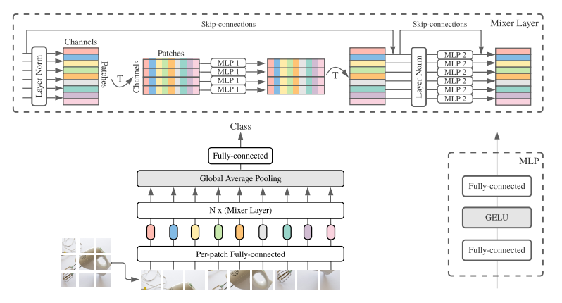
Figure 1 shows a schematic view of the MLP Mixer block, which is the main building block of the architecture. The input data for a MLP mixer has size \(P \times C\), where \(P\) is the number of patches and \(C\) is the number of channels per patch, effectively acting as a sequence of tokens. The input is first normalized through a layernorm, and then it is transposed to get a \(C \times P\) view of the data. Then the data is processed through an MLP, with the C dimension acting as a batch dimension for the purposes of the MLP. The MLP itself consists of two fully connected layers with a hidden size dependent on the size of the MLP Mixer instance and a GELU activation function. Once we get the output of the MLP block, we have a tensor where the information contained across patches corresponding to the same channel has been mixed. After this we transpose the inputs again to get back to the original \(P \times C\) size, and push them through another MLP with a similar architecture to the first one. At the end of this whole process we get back an output tensor of data with the same size as the input but with information propagated both across channels and across patches at a cost trivial in comparison to what it would be if we used a flattened image as the input to a fully connected layer.
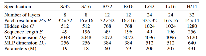
A typical configuration such as Mixer-B/16 contains 12 MLP blocks with patch resolution 16x16. The model takes 224x224 RGB images and splits them into 196 patches. Mixer-B/16 contains about 59 million parameters and achieves a throughput of 1384 images/sec/core using TPUv3, making it slightly faster than ViT-B/16 (with 861 image/sec/core using TPUv3).
When trained with large datasets and proper regularization, MLP-Mixer attains competitive performance on image classification benchmarks while keeping pre-training and inference cost comparable to state-of-the-art models. For example, when Mixer-B/16 and ViT-B/16 models were both pre-trained for 300 epochs, the ImageNet top-1 accuracy for Mixer-B/16 (76.44%) was comparable to ViT-B/16 accuracy (79.67%).
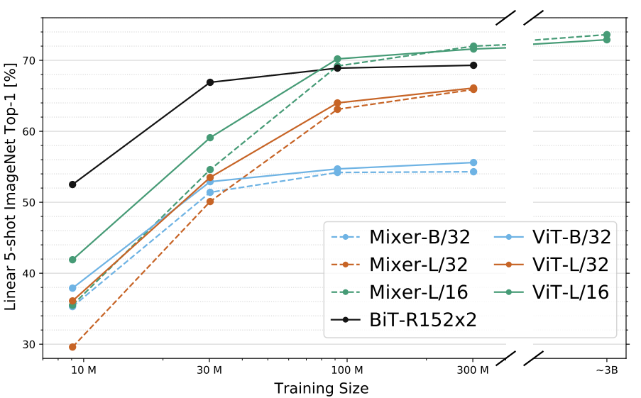
Additionally, an important factor in deciding what model to use is the scalability of the model with respect to increasing amounts of training data. The authors found that the MLP-Mixer has comparable performance to ViT as training data increases.
This paper suggests that neither convolution nor attention mechanisms are necessary to attain high performance on image classification problems. An architecture composed entirely of MLP layers can still sufficiently learn a rich feature space.
2.2 Paper 2: Caterpillar: A Pure-MLP Architecture with Shifted-Pillars-Concatenation
This paper introduces the Caterpillar architecture for computer vision tasks. The main aim is to take existing SOTA work in MLP-based architectures while reintroducing the spatial locality information that convolutions provide. To this end, the paper combines an existing MLP-based architecture, the sMLP, with a novel idea on how to inject locality. Locality is injected through a Shifted-Pillars-Concatenation (SPC) module, which acts as both a processing layer and a locality-inducing layer for the model.
The sMLP block is an architectural building block that was first introduced by Tang et al. The main idea of this block is that, instead of patching, we can use information from the row and column of a given pixel to get a better view of the context in which that pixel operates. As such, given some input tensor \(X\) with shape \(H \times W\), for each pixel at its corresponding row and columns, we project them through linear weights and concatenate them with the original pixel. The pseudocode for this operation is given by:
proj_h = nn.Linear(H, H)
proj_w = nn.Linear(W, W)
fuse = nn.Linear(3C, C)
def sparse_mlp(x):
    x_h = self.proj_h(x.permute(2,1,0)).permute(2,1,0)
    x_w = self.proj_w(x.permute(0,2,1)).permute(0,2,1)
    x = torch.concat([x_h, x_w, x], dim=2)
    x = self.fuse(x)
    return x
The sMLP block is a lot more parameter efficient than the naive MLP approach, scaling with \(N^{3/2}\) of the number of patches that we would find in an image.
The original paper introducing this block later goes on to augment it with a convolutional layer, introducing an inefficient processing step into the architecture. The Caterpillar paper aims to replace the convolutional layer with an MLP for a pure-MLP architecture. However, the original reason for why the MLP was introduced was to enrich the pixels with local information surrounding the pixel that is not present in its corresponding row and column. To this end, the paper introduces the SPC module.
The SPC module operates on a very simple idea. We can include local information surrounding a pixel in a parallelizable way by shifting the whole image by one pixel in all four directions and concatenating the pixel values from each direction into a single channel. The logic is as follows: an image of shape \(H \times W \times C\) is taken and shifted into the direction that we want to capture. We can shift every pixel up, down, left, and right depending on which direction we need. After shifting, we have to pad the image in the newly opened row or column so we still have an \(H \times W \times C\) image. Thus, we get four shifted versions of the image: \(X_u\), \(X_d\), \(X_l\), \(X_r\).
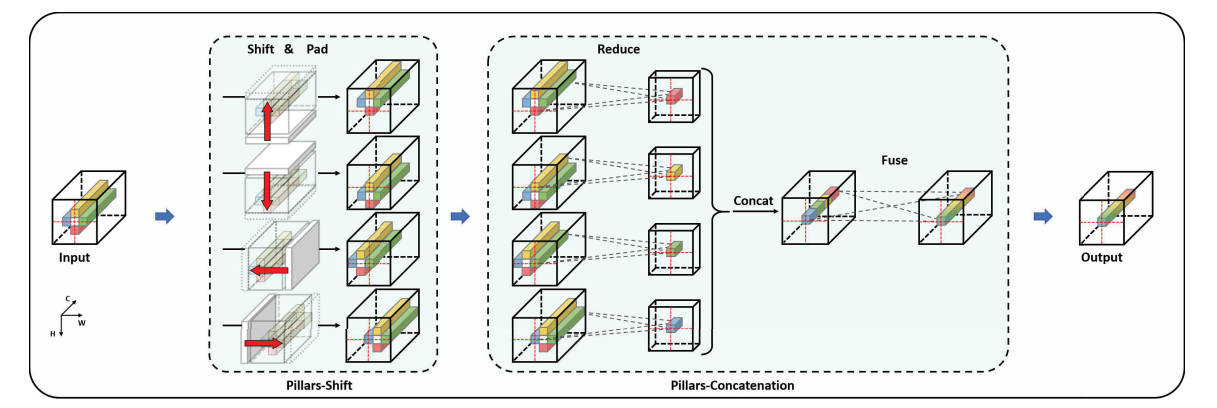
The next processing step is projecting each of these with a matrix multiplication using the corresponding learned matrix \(W_u\), \(W_d\), \(W_l\), or \(W_r\). Thus, the final output of the SPC module is given by the expression:
\[\text{SPC}(X) = \text{Concat}(X_uW_u, X_dW_d, X_lW_l, X_rW_r)W\]where \(W\) is a final projection mixing information from every shifted image.
Thus, a single Caterpillar block is given by a sequence of BatchNorm, GeLU, SPC, BatchNorm, GeLU, sMLP, LinearNorm, and MLP. The Caterpillar architecture stacks these blocks together and finally feeds the output into a classification head.
The Caterpillar architecture shows that a pure-MLP design with SPC-based locality can match or surpass strong convolutional, transformer, and hybrid baselines on both small- and large-scale benchmarks. However, the most interesting evaluation shown by the authors was in taking the standard ResNet architecture and swapping out convolutions with SPC blocks. This yielded up to a 4.7% performance improvement for a ResNet-18-style architecture, showing that the MLP-only architecture is capable of fully replacing and outperforming convolutions at similar sizes.
2.3 Paper 3: ResMLP: Feedforward networks for image classification with data-efficient training
ResMLP is an architecture that is built entirely based on MLPs. ResMLP contains two blocks, the cross-patch sublayer and cross-channel sublayer. The cross-patch linear layer is applied to all channels independently, to mix across patches. The cross-channel sublayer is applied independently to all patches, to mix information locally.
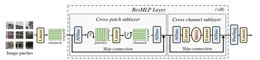
In ResMLP, images are first split into \(N \times N\) non-overlapping patches (usually 16x16). The patches are independently passed through a linear layer to form a set of \(N^2\) \(d\)-dimensional embeddings. These embeddings are passed into the ResMLP layer. Each sublayer of the ResMLP layer runs in parallel with a residual connection. The first step is an Affine transformation defined by:
\[\text{Aff}_{\alpha, \beta}(x) = \text{Diag}(\alpha)x + \beta\]Where \(\alpha\) and \(\beta\) are learnable weight vectors. The embeddings are then passed into a linear layer after transposing to mix across patches. It is transposed back to receive the original shape before the first affine transformation, and fed into a different affine transformation. The affine transformation at the beginning (pre-normalization) is initialized with \(\alpha = 1\) and \(\beta = 0\). The affine transformation at the end of the residual block (post-normalization) is initialized with a small \(\alpha\) value. These embeddings are recombined with its residual connection and fed into the cross-channel sublayer. The cross-channel sublayer follows a similar layout with affine transformations in the beginning and end of the sublayer. In the middle, two linear layers separated by GeLU activation function are present. Lastly an average pooling is done the d-dimensional patches and fed into a linear classifier to predict a label associated with the image. The ResMLP Layer can be described by the following:
\[Z = X + \text{Aff}((A \cdot \text{Aff}(X)^T)^T)\] \[Y = Z + \text{Aff}(C \cdot \text{GeLU}(B \cdot \text{Aff}(Z)))\]where \(A\), \(B\), \(C\) are learnable weight matrices. One baseline model is the ResMLP-S12 model. It contains 12 ResMLP blocks with patch resolution \(16 \times 16\). The model takes \(224 \times 224\) RGB with hidden dimension \(384\). This model takes 1.54 million parameters and has a throughput of 1415.1 image/sec, where DeiT-S had a throughput of 940.4 images/sec when trained on a single V100-32GB GPU with batch size of \(32\).
ResMLP attains similar accuracy to Transformers and Convolution networks. For example, when ResMLP-S12, EfficientNet-B3, and DeiT-S models were pre-trained on ImageNet, top-1 accuracy for ResMLP-S12 (76.6%) came very close to both EfficientNet-B3 accuracy (81.1%) and DeiT-S accuracy (79.8%).
The ResMLP architecture demonstrates that a purely MLP design using the combination of residual connections and affine transformations can reach SOTA performance with significantly higher throughput.
Methodology Comparison
3.1 Structural Approaches to “Mixing” Information
The three papers that we presented all try to grapple with the problem of inductive bias when working with image data. Convolutions, even though they may be computationally inefficient, have a very strong inductive bias towards locality. Locality is a very useful inductive bias for image data, so adding it into a model architecture is a central problem in designing models for computer vision. MLPs do not natively have any kind of inductive bias, so the presented papers all try to introduce locality bias to reach SOTA performance as well as get the improved computational efficiency of MLPs.
The MLP mixer and ResMLP models have locality built into them through the per-patch MLP processing. These models have a \(P \times C\) shaped input, where \(P\) is the number of patches and \(C\) is the number of channels per patch. When we run this input through an MLP across the \(P\) dimension, the MLP processes each patch individually, meaning it sees all the local information in the patch. This process introduces strong inductive bias towards locality.
The Caterpillar model has a different approach. The original paper introducing Caterpillar’s main MLP module, the sMLP, used convolutions in their main processing block to introduce locality. However, the Caterpillar models use a shifted pillars concatenation method, which takes each pixel’s neighbors and concatenates all of the data contained within those neighbors into a single local feature. This is then processed by the sparse MLP, which now sees local information surrounding each pixel.
3.2 Model Architectures and Dimensionality
The three presented models all approach the data processing from different sides. The MLP-Mixer model treats input images as sequences of tokens, whereas the Caterpillar model has a different approach that focuses on modifying the content of pixels inside a feature map through shifting, padding, and looking at rows and columns of the feature map.
These models also take different approaches to normalization. MLP-Mixer utilizes Layer Norms for normalization before every mixing step. The ResMLP model takes this a step further, by introducing a special learned affine transformation both as a pre and post normalization to manage the signal propagation through the network without using BatchNorm or LayerNorm in its computational blocks. The Caterpillar model uses BatchNorm combined with GeLU activation in its own block structure. Thus, each of these models have a unique way of normalizing the inputs to their processing blocks to manage how well gradients can propagate and data can be processed inside them.
The models also take different approaches when it comes to the reduction and expansion of the representation of its input data. MLP-Mixer and ResMLP patch the input images and run their respective MLPs across the resized data while keeping the overall size constant throughout the process. Caterpillar projects the shifted pixel data it creates via matrix multiplication thus in some way having a similar idea to the channels of convolutional layers.
3.3 Training Strategies & Datasets
The MLP-Mixer model requires large datasets and regularization to learn, reminiscent of transformer models. Also similarly to transformer models, it has been shown to scale linearly with data volume, tracking ViTs very closely in performance vs data graphs.
The ResMLP was explicitly designed to be as data-efficient as possible, utilizing specific initializations for both their MLPs and their affine transformation to make gradient flows stable and efficient.
3.4 Evaluation Metrics
The promise of MLP based models is that they could harness the efficiency of large parallelized matrix multiplications, while not compromising on model performance. Thus, the metrics presented in the papers as well as the metrics we focus on in this literature review are the throughput/inference speed and accuracy, with accuracy being important but somewhat secondary to throughput as long as it is at a similar level to the SOTA.
All of the presented models have been shown to be able to reach near-SOTA performance at much lower processing cost and much higher throughput. MLP-Mixer B/16 is able to process over 1300 images per second per core on the TPUv3 hardware, compared to the 280 images per second per core for the ViT model, at only 5% less accuracy for ImageNet. ResMLP also shows this extremely high computational efficiency, reaching over 1400 images per second on the V100 GPU. These performance numbers are a function of MLPs being able to utilize the hardware acceleration focus of GPUs on matrix multiplication, allowing them to reach much closer to the peak FLOPs of the utilized hardware than convolution based networks. Thus, all the models presented here have shown that one could harness both computational advantages of the MLP as well as get high accuracy on the modeling tasks.
4. Results and Performance Comparison
4.1 Accuracy against SOTA Baselines
Results for the MLP-Mixer model, especially when compared with the Vision Transformer, indicate that the MLP architecture can achieve accuracy comparable to the attention-based models while being significantly faster. The Mixer-B/16 model was trained to match the ViT-B/16 model’s 300 epochs of pre-training, with the MLP-Mixer achieving a 76.44% accuracy. This is competitive but slightly lower than the accuracy achieved by the ViT, which was 79.67%. This suggests that the ViT adds some inductive biases through the attention mechanism that are not present in the MLP-mixer’s approach.
The ResMLP model shows a similar trend. The ResMLP-S12 model achieves a Top-1 accuracy of 76.6% on ImageNet, which brings it close to the convolution-based EfficientNet-B3 and transformer-based DeiT-S models. One thing that we must remember, however, is that the convolution and transformer models are highly optimized and engineered, making the near-SOTA performance of the MLP based model more encouraging. This is achieved while being faster than both the EfficientNet and DeiT models.
The Caterpillar model measures a very interesting effect. One question asked by the paper is, what if we took an existing convolution based model and swapped out the convolution for a MLP-based module. The Caterpillar work modified the ResNet-18 architecture with their shifted pillars concatenation blocks to observe the performance change with respect to the original ResNet-18. The modification resulted in a performance improvement of up to 4.7%. This gain highlights the potential of the SPC module as a pure MLP-based module to introduce important inductive biases into architectures while still harnessing the computational efficiency of large matrix multiplications.
4.2 Computational Efficiency and Hardware Alignment
As we stated earlier, accuracy is not the only metric that we would like to address here. An arguably more important metric for the purposes of this analysis is the computational efficiency of the models. Here, MLP-based architectures have a clear advantage due to their structure. For example, the Mixer-B/16 model achieved a throughput of 1384 images per second per core on the TPUv3. This can be compared to the ViT-B/16 model which has a processing speed that is 38% slower. This efficiency gap generalizes to the ResMLP architecture, where the ResMLP-S12 achieves a throughput speed that is over 30% faster than the DeiT-S model on the V100 GPU. These metrics show what we posited originally, that the hardware architecture of GPUs and TPUs, as well as the amount of optimization that goes into matrix multiplication, makes MLPs a clear advantage in speed.
This advantage in speed is also easier to scale through optimization. The current hardware architectures lend themselves very easily to multi-precision processing. Matrix multiplication is one of the easiest operations to implement for native INT8 and FP4 precisions, which makes both the processing time more than double, and the memory movements of the large matrices significantly faster. Thus, MLPs being an architecture that uses matrix multiplication very heavily, makes them perfect for fast inference and efficient training, especially compared to convolutions.
5. Cross-Paper Analysis
One of the implied consequences of the MLP-based approach to modeling is the rejection of the large importance of inductive bias. This includes both the local inductive bias of convolutions, and global inductive bias of transformers. Each architecture is built mostly on the premise that a rich feature space can be learned through matrix multiplications without large inductive biases. Of course, this conclusion is limited to an extent by the architecture of the models, which in all three cases attempts to encode some inductive biases through either the approach to patch processing for MLP-Mixer and ResMLP, or the SPC module for the Caterpillar model. Regardless, however, the inductive bias introduced by these techniques are significantly less strong than those encoded in transformers and convolutions.
The different attempts to encode said inductive biases have some interesting differences as well as similarities between the models. The MLP-Mixer and ResMLP models approach locality through mixing local information within patches with global information across patches. The ResMLP model additionally utilizes the affine transformation to handle signal propagation through this locality-inducing operation. The Caterpillar model approaches locality very differently. There is no patching for the Caterpillar model, but rather explicit locality introduced through features from spatial neighbors of a given pixel being concatenated together into a single feature vector. While this seems to be a very explicit inclusion of locality as inductive bias, it is not nearly as strong as the inductive bias encoded in convolutional layers. Thus the three models reject strong inductive biases in favor of weaker biases coupled with dense matrix multiplications as the primary modeling approach. While this gets the models most of the way to SOTA performance, some gains are still required to show complete equivalence of performance to current SOTA approaches with stronger inductive biases.
These differences in approach are, mostly, orthogonal to each other. As shown by Caterpillar, one can get large performance gains through adding SPC based modules to existing models like the ResNet-18. This suggests that integrating an SPC-like method into the MLP-Mixer or ResMLP could lead to performance superior to the original models. Additionally, the insight gained through ResMLP’s use of affine transformations in place of normalization is also possible to leverage in designing MLP based models. In principle, the affine transformation can be simply put into place instead of BatchNorm or LayerNorm in the other models. Finally, it is important to recognize the differences in scale in these models. The ResMLP model is a highly parameter-efficient model, showing that MLP based models can achieve good performance with few parameters. In contrast, MLP-Mixer shows that MLPs can scale at least as well as vision transformers with the amount of data, training compute, and number of parameters.
6. Conclusion
This literature review explored three MLP-based architectures, the MLP-Mixer, ResMLP, and Caterpillar. The aim of the review was to show that MLP-based architectures can reach near-SOTA performance, while having more efficient hardware utilization and faster inference. This thesis is largely supported by the data found in the papers.
The presented methods reach accuracies on ImageNet that are within 5% of comparable-sized SOTA models, and within 10% of overall SOTA. The MLP-Mixer model achieves an accuracy of over 76% on ImageNet, compared to similarly sized ViT-B’s 79%. This shows the accuracy part of our thesis to be valid. Additionally, the authors report an over 30% increase in throughput compared to the same model, showing that the theoretical performance gains that come with such a matrix multiplication heavy model can materialize into large actual speedups.
7. References
[1] LeCun et al., “Gradient-Based Learning Applied to Document Recognition,” 1998.
[2] Krizhevsky et al., “ImageNet Classification with Deep Convolutional Neural Networks,” 2012.
[3] He et al., “Deep Residual Learning for Image Recognition,” 2016.
[4] Kingma & Ba, “Adam: A Method for Stochastic Optimization,” 2015.
[5] Han et al., “Learning Both Weights and Connections for Efficient Neural Networks,” 2015.
[6] Dosovitskiy et al., “An Image is Worth 16×16 Words: Transformers for Image Recognition at Scale,” 2021.
[7] “Vision Transformer,” Wikipedia.
[8] Tolstikhin et al., “MLP-Mixer: An All-MLP Architecture for Vision,” 2021.
[9] Liu et al., “Are We Ready for a New Paradigm Shift? A Survey on Visual Deep MLP,” 2022.
[10] Sun et al., “Caterpillar: A Pure-MLP Architecture with Shifted-Pillars-Concatenation,” 2024.
[11] Touvron et al., “ResMLP: Feedforward networks for image classification with data-efficient training,” 2021.