Streetview Semantics
[Project Track] Street-level semantic segmentation is a core capability for autonomous driving systems, yet performance is often dominated by severe class imbalance where large categories such as roads and skies overwhelm safety-critical but rare classes like bikes, motorcycles, and poles. Using the BDD100K dataset, this study systematically examines how architectural choices, loss design, and training strategies affect segmentation quality beyond misleading pixel-level accuracy. Starting from a DeepLabV3-ResNet50 baseline, we demonstrate that high pixel accuracy (~ 94%) can coincide with extremely poor mIoU (~ 4%) under imbalance. We then introduce class-weighted and combined Dice-Cross-Entropy/Focal losses, auxiliary supervision, differential learning rates, and gradient clipping, achieving a 10x improvement in mIoU. Then, we propose a targeted optimization strategy that remaps the task to six safety-critical small classes and leverages higher resolution, aggressive augmentation, and boosted class weights for thin and small objects. This approach significantly improves IoU for bicycles, motorcycles, and poles, highlighting practical trade-offs between accuracy, resolution, and computational cost. However, such increases in resolution resulted in significant increases to training time per epoch, resulting in less training. Our last contribution is a boundary-aware auxillary supervision strategy that explicitly promotes boundary preservation for thin and small objects while maintaining architectural simplicity. Overall, the work provides an empirically grounded blueprint for addressing class imbalance and small-object segmentation in urban scene understanding.
Streetview Semantics
What is streetview semantics?
Streetview semantics involves assigning meaningful labels such as road, sidewalk, building, vehicle, pedestrian, or sky to pixels or regions in images captured from a street-level perspective.
Semantic segmentation of streetview images can be used to transform raw visual input into a structured representation, where each region corresponds to an object or surface with a specific functional role. This semantic understanding enables higher-level reasoning about the environment, such as identifying drivable areas, detecting obstacles, and interpreting relationships between objects in down stream tasks, like autonomus driving.
Dataset
The BDD100K dataset [2] includes a diverse collection of streetview images designed for autonomus driving research. The dataset includes images captured by a camera mounted on a vehicle from a variety of locations like New York and San Francisco.
We use 10,000 images and their semantically segmented labeled masks to train and test our model.
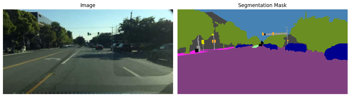 A sample image and its corresponding mask from the dataset.
| Class | Pixel Count | Percentage |
|---|---|---|
| Road | 14,112,633 | 26.43% |
| Sidewalk | 1,072,369 | 2.01% |
| Building | 8,773,136 | 16.43% |
| Wall | 300,296 | 0.56% |
| Fence | 520,512 | 0.97% |
| Pole | 635,225 | 1.19% |
| Traffic light | 81,342 | 0.15% |
| Traffic sign | 284,603 | 0.53% |
| Vegetation | 8,817,392 | 16.51% |
| Terrain | 725,905 | 1.36% |
| Sky | 11,134,137 | 20.85% |
| Person | 187,644 | 0.35% |
| Rider | 16,331 | 0.03% |
| Car | 5,684,376 | 10.65% |
| Truck | 622,560 | 1.17% |
| Bus | 401,880 | 0.75% |
| Train | 8,826 | 0.02% |
| Motorcycle | 7,140 | 0.01% |
| Bicycle | 10,650 | 0.02% |
Table 1: Pixel distribution across semantic classes in the dataset.
The BDD100K dataset exhibits severe class imbalance, with a small number of large classes; most notably road, vegetation, and sky-dominating pixel coverage, while many semantically and operationally important classes occupy only a minimal fraction of the image area. This imbalance induces a common failure mode in semantic segmentation, whereby models achieve high pixel-level accuracy by overpredicting majority classes while largely ignoring rare objects. Such behavior is particularly problematic in autonomous driving contexts, where small and thin objects such as bicycles and poles are both visually challenging and safety-critical. Accordingly, our objective is not to optimize global accuracy, but to improve the reliable detection and segmentation of minority classes relative to a baseline, even when this entails trade-offs on dominant classes.
Initial baseline implementation
We first started with simply feeding our test set to DeepLabV3 [1] with a ResNet-50 Backbone [5].
We chose this model for its proven performance on urban scene understanding (Cityscapes [6], COCO), its Atrous Spatial Pyramid Pooling (ASPP) module for multi-scale context, pretrained ResNet-50 backbone for strong feature representations, and auxiliary classifier head for improved gradient flow.
Our initial model performed deceptively well (when it was in fact not performant at all) because we used pixel-level accuracy as our metric. When checking model predictions on the test set, we can see the model is not performing well:
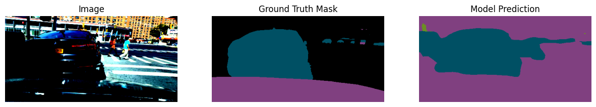
High pixel accuracy: ~ 93%
Very poor mIoU: ~ 4%
This was likely caused by a severe class imbalance in the BDD100K dataset. The model learns to predict only common classes, causing high pixel accuracy but poor mIoU.
Improvements atop Baseline Model
We implemented a variety of additions to our baseline model in hopes of pushing the model to classify low-density classes more.
1. Class Weighting
We assign higher weight to rarer classes (less pixels labeled in pictures in the dataset) in our loss function in order to get our model to focus on these fine grained details. This prevents the model from straight out ignoring minority classes and simply labeling majority classes to everything. This works as a sort of increased penalty for cheating.
We assign inverse-frequency weight for class \(f_c\) and normalize.
\[w_c = \frac{\frac{1}{f_cC}}{\sum_{i=1}^C w_i}C\]2. Combined Loss Function
We use a combined Dice loss and Cross Entropy loss to better handle the class imbalance and improve boundary predictions.
Dice loss is defined as:
\[{L}_{d} =1 - \frac{2\sum_{i=1}^n y_{pred_i}y_{true_i} + \epsilon}{\sum_{i=1}^n y_{pred_i} + \sum_{i=1}^n y_{true_i} + \epsilon}\]Cross Entropy loss is defined as:
\[{L}_{CE} = -\sum_{c=1}^N y_clog(p_i)\]The combined loss is simply
\[{L} = {L}_{d} + {L}_{CE}\]This creates a training objective that balances per-pixel classification accuracy and region level overlap, encouraging accurate semantic prediction.
3. Auxiliary Loss Usage
We make use of the two predictions the network produces: full-resolution prediction and the intermediate aux_out prediction from an earlier layer. This helps our deep network’s gradients have a shorter path to reach earlier layers.
main_loss = criterion(main_out, masks)
aux_loss = criterion_aux(aux_out, masks)
total_loss = main_loss + 0.4 * aux_loss
4. Separate Learning Rates
| Parameter Group | Learning Rate | Weight Decay |
|---|---|---|
| Backbone Parameters | 1e-4 | 1e-4 |
| Classifier Parameters | 1e-3 | 1e-4 |
We reduce the learning rate of the pretrained backbone and increase it for the classifier head to allow for better retainment of high-level vision understanding while better learning our dataset.
5. Gradient Clipping
We clip gradients to a max norm of 1 to prevent exploding gradients. This allows for more stable training.
\[g_i \leftarrow g_i \frac{1}{||\textbf{g}||_2}\]Further Model Development
The initial results of running our model through 6400 training samples on 9 epochs produced best model at the 9th epoch with validation mIoU (on 1600 test samples) of 41.56%.
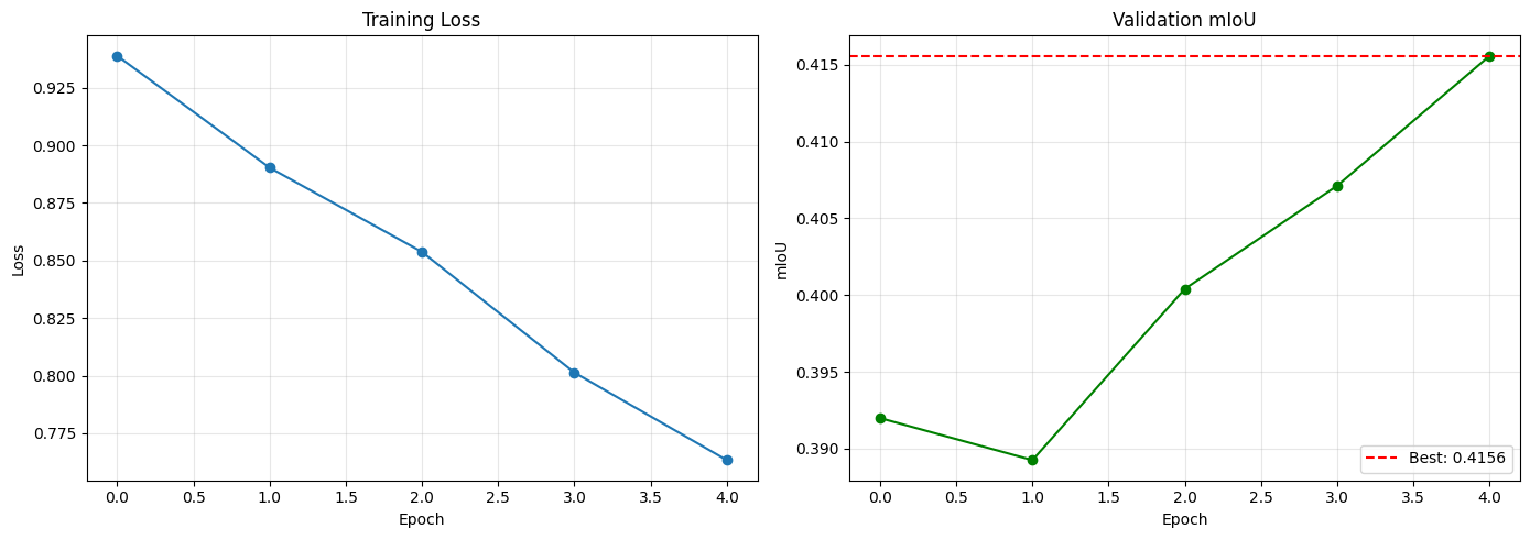 Note that the Epoch axies are wrong here; we trained 4 extra epochs after it was already trained for 5.
This shows promising improvement over our baseline. Looking at some model sample outputs, we see the model is able to identify large segments but struggles to match a precise boundary.
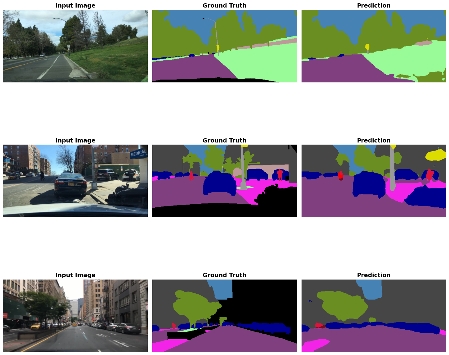
This is reflected in our model’s per-class mIoU:
| Class | IoU |
|---|---|
| road | 0.6055 |
| sidewalk | 0.4564 |
| building | 0.6682 |
| wall | 0.2186 |
| fence | 0.3026 |
| pole | 0.2435 |
| traffic_light | 0.3113 |
| traffic_sign | 0.3164 |
| vegetation | 0.7488 |
| terrain | 0.3584 |
| sky | 0.8786 |
| person | 0.4281 |
| rider | 0.2265 |
| car | 0.7943 |
| truck | 0.4343 |
| bus | 0.5171 |
| train | 0.0010 |
| motorcycle | 0.2024 |
| bicycle | 0.1842 |
mIoU: 0.4156
In order to test whether our model can effectively differentiate difficult classes, however, we decided to repeat the same training setup using a modified dataset. In this variant, all classes are assigned a weight of 0 except for pole, vegetation, person, car, motorcycle, and bicycle. These classes are suspected to be especially difficult to segment due to their low frequency in the dataset and, for some, their thin or fine-grained structure.
The resulting model performed significantly worse overall, with particularly poor performance on thin objects such as poles, motorcycles, and bicycles with individual IoUs of less than 0.001 and an overall mIoU of 25%.
This collapse in our first 6-class attempt pushed us to design a third version: moving to 1024 x 512 resolution, stronger Focal Loss [3] focus (y = 3.0), heavier class weights (bike/moto 3x, pole 2x), wider scale augmentation (0.5 - 2.0), tighter crops (0.6 - 1.0) to keep small objects in frame, and light random erasing to cut background reliance. The combined Focal Loss [3] and Dice Loss [4] formulation helped target hard examples and improve boundary predictions for thin objects. The goal was to recover and improve thin-object performance, especially for bicycles and motorcycles, while staying focused on the six safety-critical classes. However, these improvements, especially the increase in resolution did lead to a significant increase in training time (one hour per epoch) as we would need to half the batch size.
After 10 epochs with the improved v3 setup, the 6-class evaluation produced the following class-wise weights and IoU scores:
| Class | Weight | IoU |
|---|---|---|
| pole | 0.233 | 0.0105 |
| vegetation | 0.100 | 0.6153 |
| person | 0.817 | 0.4454 |
| car | 0.100 | 0.7371 |
| motorcycle | 10.000 | 0.2537 |
| bicycle | 7.243 | 0.0934 |
mIoU: 0.3592
Although our overall mIoU was still lower than our model for all classes, it still showed significant improvement as not only were pole and bicycle able to break the 0.01 value of IoU, motorcycle improved drastically , reaching an IoU of 0.25. However we do believe that further training could generate even stronger results.
Model Development Versions
Model v1 - Baseline DeepLabV3
Architecture: DeepLabV3-ResNet50 pretrained on COCO
Configuration:
- Resolution: 512 x 256
- Classes: All 19 BDD100K classes
- Loss: Cross Entropy only
- Batch Size: 8
Performance:
- Pixel Accuracy: ~ 94%
- mIoU: ~ 4%
Key Problem: Severe class imbalance - road and sky dominate
Model v2 - Class Balancing & Loss Improvements
Improvements over v1:
- Class weighting
- Combined Focal Loss
- Auxiliary loss branch
- Separate learning rates
- Gradient clipping
Configuration:
- Resolution: 512 x 256
- Classes: All 19 BDD100K classes
- Loss: Focal (y = 2.0) + Dice (weight = 0.3)
- Batch Size: 8
- Epochs: 10
Performance on all 19 classes:
- Pixel Accuracy: ~ 88 - 92%
- mIoU: ~ 40%
- Common: ~ 80%
- Medium: ~ 50%
- Rare: ~ 20%
Performance on just 6 classes:
- mIoU: ~ 20%
- Bicycles, Motorcycles, Poles: ~1%
Model v3 - Bicycle/Motorcycle Targeted Optimization
Approach: Focused optimization on 6 safety-critical urban classes with emphasis on thin/small objects
Key Improvements over v2:
- Doubled Resolution
- 1024 x 512 (4x pixels)
- Critical for thin objects (bicycles, motorcycles, poles)
- Improved small object segmentation
- Enhanced Focal Loss
- Gamma: y = 3.0
- Stronger focus on hard negatives
- Better handles misclassified edge pixels
- Class Weight Boosting
- Bicycle: 3.0x base weight
- Motorcycle: 3.0x base weight
- Pole: 2.0x base weight
- Prevents model from ignoring safety-critical minority classes
- Wider Scale + Object-Centric Crops
- Scale range: 0.5 - 2.0x
- Random crop 0.6 - 1.0x to keep small/thin objects in view
- Gaussian blur, color jitter for robustness
- Combined Loss Refinement
- Focal Loss (y = 3.0): Hard example mining
- Dice Loss (weight = 0.3): Boundary prediction
- Complementary benefits for small objects
- Light Random Erasing (train only)
- p = 0.3, small holes to reduce background reliance
- Encourages robustness to occlusion and clutter
Configuration:
- Resolution: 1024 x 512
- Classes: 6-class subset (bicycle, motorcycle, pole, car, person, vegetation)
- Loss: Focal (y = 3.0) + Dice (weight = 0.3)
- Batch Size: 4
- Epochs: 10
Performance:
- mIoU: ~ 36%
- pole: ~ 1%
- vegetation: ~ 62%
- person: ~ 45%
- car: ~ 74%
- motorcycle: ~ 25%
- bicycle: ~ 9%
Boundary-Aware Auxiliary Supervision
Recent research has proposed incorporating explicit boundary or edge information into semantic segmentation models. The motivation behind these approaches is that by introducing an auxiliary task that supervises object boundaries, the model can learn finer-grained spatial features that improve the distinction between adjacent objects.
Related Work
We draw inspiration from Takikawa et al., who proposed Gated-SCNN: Gated Shape CNNs for Semantic Segmentation (ICCV 2019) [6]. Their work demonstrates that incorporating boundary and shape prediction objectives significantly improves both mean Intersection-over-Union (mIoU) and boundary F-score, with particularly strong gains for thin and small objects. While effective, this approach requires substantial architectural changes and increased computational cost, as it introduces a two-stream CNN architecture.
Our Design
In our work, we adopt explicit boundary supervision as an auxiliary task. Rather than modifying the core architecture, we augment the model with a lightweight boundary prediction head and an additional loss term during training. Boundary labels are generated directly from the ground-truth segmentation masks, requiring no additional annotations. A pixel is labeled as a boundary pixel if any of its 4-connected neighbors belongs to a different semantic class (excluding ignore regions). This produces a binary boundary map in which pixels on class transitions are marked as 1, and all other pixels are marked as 0. This process is deterministic, computationally inexpensive, and ensures perfect alignment between segmentation and boundary targets.
To incorporate boundary supervision into the model, we attach a small boundary prediction head to the shared feature representation produced by the Atrous Spatial Pyramid Pooling (ASPP) module. Specifically, a 1×1 convolutional layer is added on top of the ASPP features to predict a single-channel boundary logit map. The segmentation head and boundary head share all upstream features, enabling multi-task learning without duplicating computation. Importantly, the DeepLabv3 backbone and ASPP remain unchanged. To avoid modifying the model’s output interface, ASPP features are accessed via a forward hook, preserving the original training and evaluation pipeline.
This design was chosen to balance effectiveness and simplicity. Attaching the boundary head at the ASPP level allows the auxiliary task to operate on high-level semantic features while still retaining sufficient spatial resolution for boundary localization. In contrast, attaching boundary supervision earlier in the backbone would emphasize low-level edge detection but was found to produce noisier boundary predictions that did not align well with semantic class transitions. Using a lightweight 1×1 convolution further minimizes additional parameters, reducing the risk of overfitting and ensuring that performance gains arise from improved supervision rather than increased model capacity.
Loss Function
The total training objective is defined as:
\[ L = L_{\text{seg}} + \lambda L_{\text{boundary}} \]
Here, L_seg denotes the primary segmentation loss from before, implemented as a combination of focal loss and Dice loss to address class imbalance and improve region-level overlap. The boundary loss L_boundary is defined as a binary cross-entropy loss with logits, applied only to valid (non-ignore) pixels and computed from boundary targets derived from ground-truth segmentation masks. The scalar weight lambda controls the relative contribution of boundary supervision and is set to 0.2. Empirically, we found that this weighting provides a good trade-off between encouraging precise boundary localization and maintaining region-level semantic consistency. Larger values of lambda tended to overemphasize fine-grained edges at the expense of interior region accuracy, while smaller values diminished the impact of the auxiliary task.
Results
| Class | IoU |
|---|---|
| pole | 0.2958 |
| vegetation | 0.7590 |
| person | 0.4829 |
| car | 0.8043 |
| motorcycle | 0.2450 |
| bicycle | 0.0010 |
mIoU: 0.3817
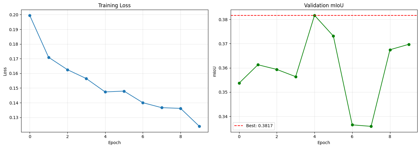 Training and validation metrics for the boundary-aware model.
Note that the validation graph indicates optimization instability with its mild fluctuations.
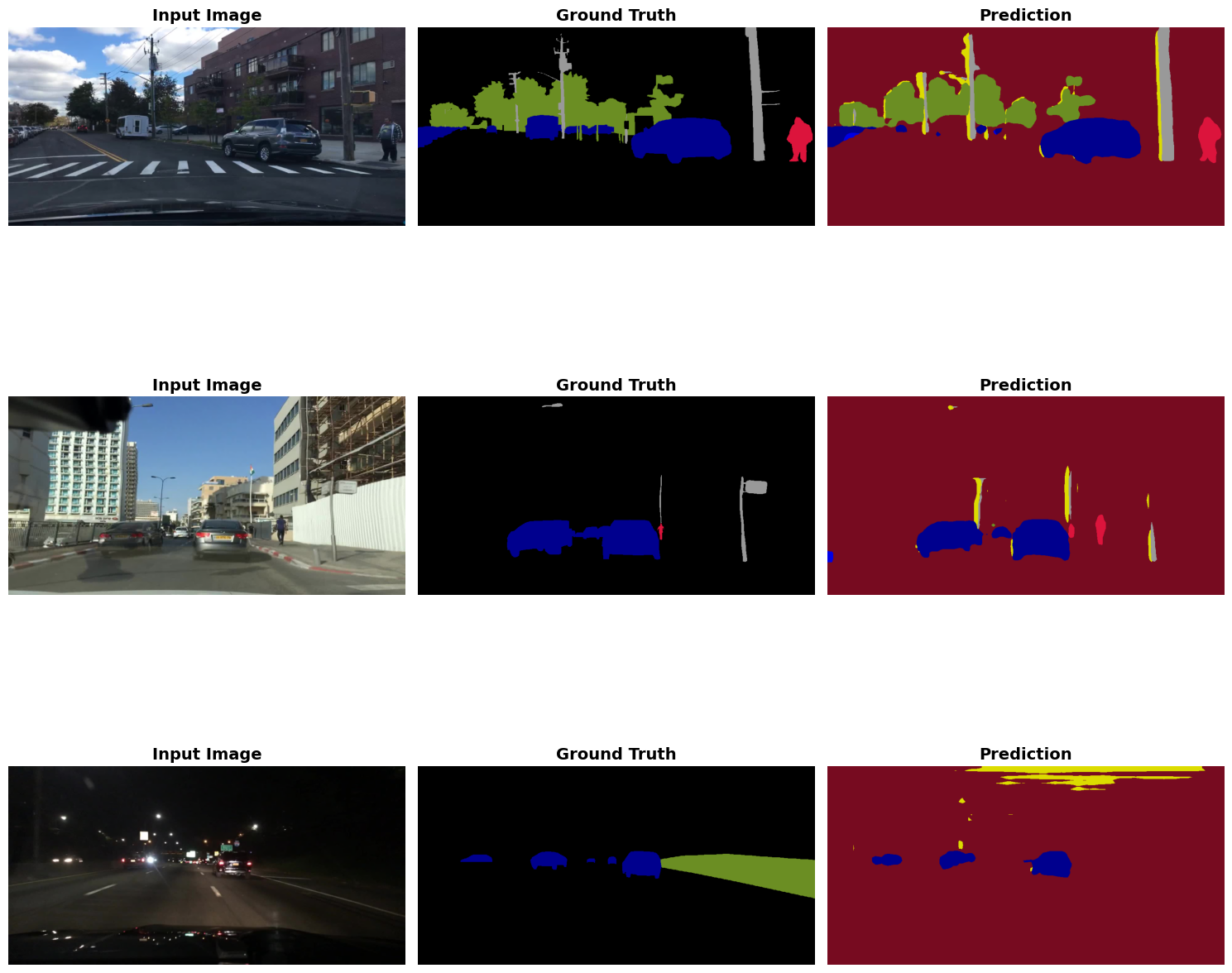 Sample segmentation outputs from the boundary-aware model showing improved boundary preservation.
The boundary-aware model improves overall performance, increasing mIoU from 0.3592 (DeepLabv3 baseline) to 0.3817. The largest gains occur for boundary-sensitive classes, most notably pole, which improves from 0.0105 to 0.2958, demonstrating the effectiveness of explicit boundary supervision for thin structures. Improvements are also observed for vegetation (0.6153 → 0.7590), car (0.7371 → 0.8043), and person (0.4454 → 0.4829). Note that our additions seemed to improve for large objects as well,
Performance on motorcycle remains largely unchanged, while bicycle exhibits a decrease in IoU. This suggests that although boundary supervision improves localization, it may overemphasize edges for extremely sparse objects without sufficiently reinforcing interior regions. Overall, these results validate boundary-aware auxiliary supervision as an effective and lightweight improvement over the baseline, particularly for thin and boundary-sensitive classes.
As future work, more experimentation would be necessary to evaluate how our boundary-aware auxiliary supervision improves all class IoUs or fine-grained structures disproportionately. Additionally, exploring complementary approaches such as region-consistency losses, shape-aware architectures, or post-processing refinement methods may further improve performance on challenging small and thin object classes.
Future uses
Beyond standard IoU metrics, we implemented a RoadSafetyAnalyzer class in our notebook that computes a composite safety score (0 - 100) based on segmentation predictions. This scorer evaluates road visibility, pedestrian and vehicle presence, obstacle detection, and lane clarity to provide a risk-level assessment (LOW, MODERATE, HIGH, CRITICAL) for each scene.
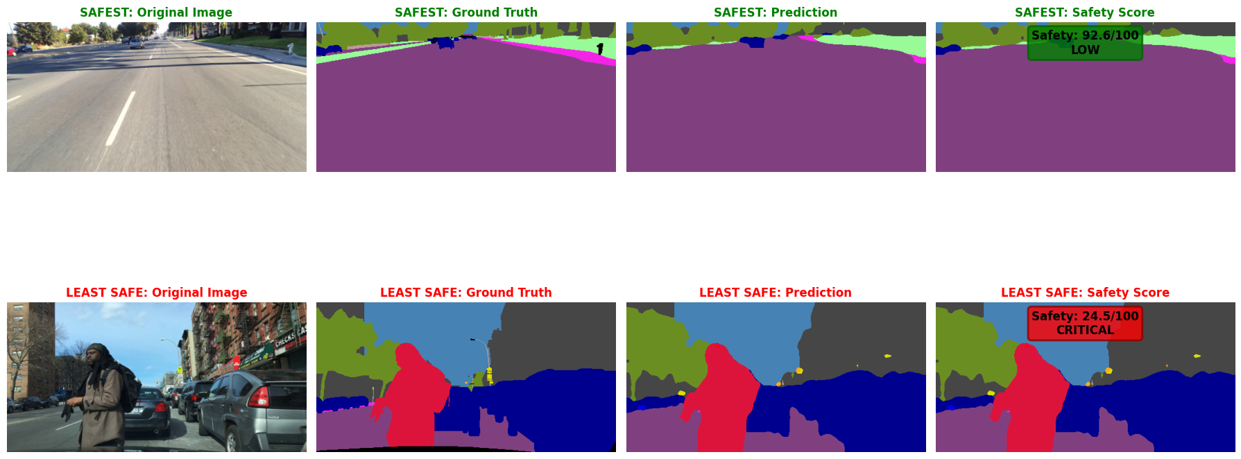
Future work could extend this framework to temporal analysis across video sequences, multi-sensor fusion, and adaptive policy generation based on safety scores.
Conclusion
This work demonstrates that semantic segmentation performance in urban driving scenes cannot be meaningfully assessed, or improved, using pixel-level accuracy alone in the presence of extreme class imbalance. Through a series of controlled model iterations on the BDD100K dataset, we show that loss design, class-aware weighting, and training strategy play a decisive role in recovering minority-class performance. By progressively shifting from a general-purpose baseline to a targeted, high-resolution optimization focused on safety-critical classes, and explicitly encouraging boundary preservation, we achieve substantial gains in mIoU and per-class IoU for thin and rare objects such as poles and other fine-grained structures. These results highlight the necessity of task and risk-aware model design in autonomous driving and provide a practical blueprint for addressing imbalance-driven failure modes without reliance on dataset expansion.
References
[1] Chen, L. C., Papandreou, G., Schroff, F., & Adam, H. “Rethinking atrous convolution for semantic image segmentation.” arXiv preprint arXiv:1706.05587. 2017.
[2] Yu, F., Chen, H., Wang, X., Xian, W., Chen, Y., Liu, F., … & Darrell, T. “BDD100K: A diverse driving dataset for heterogeneous multitask learning.” Proceedings of the IEEE/CVF conference on computer vision and pattern recognition. 2020.
[3] Lin, T. Y., Goyal, P., Girshick, R., He, K., & Dollar, P. “Focal loss for dense object detection.” Proceedings of the IEEE international conference on computer vision. 2017.
[4] Milletari, F., Navab, N., & Ahmadi, S. A. “V-net: Fully convolutional neural networks for volumetric medical image segmentation.” 2016 fourth international conference on 3D vision (3DV). 2016.
[5] He, K., Zhang, X., Ren, S., & Sun, J. “Deep residual learning for image recognition.” Proceedings of the IEEE conference on computer vision and pattern recognition. 2016.
[6] T. Takikawa, D. Acuna, V. Jampani and S. Fidler, “Gated-SCNN: Gated Shape CNNs for Semantic Segmentation,” 2019 IEEE/CVF International Conference on Computer Vision (ICCV), Seoul, Korea (South), 2019.