Unupervised Domain Adaptation with GTA -> Cityscapes
Introduction
Imagine spending millions of dollars training a self-driving car in the streets of California, only to watch it fail when deployed on the streets of London. Or picture an autonomous vehicle that performs flawlessly in video game simulations like GTA5, but can’t recognize a simple stop sign when it encounters real-world weathering and reflections. This is one of the most critical challenges facing computer vision today: the domain gap.
The field of domain adaptation attempts to handle this problem of different distributions of data in computer vision. Under supervised learning, deep learning models excel when training and testing data come from the same distribution. Train a segmentation model on synthetic data, and it achieves near-perfect accuracy on more synthetic data. But the moment you deploy it in the real world, performance plummets. Roads become unrecognizable, pedestrians vanish, and traffic signs blur into the background. This is due to the model having overfit to the training data. The task therefore is to minimize the discrepancy between performance on the source domain and the target domain.
Over the past decade, researchers have developed increasingly sophisticated techniques to bridge this domain gap. Our blog will examine the specific focus of unsupervised domain adaptation (UDA) from training on GTA5 to performance on CityScapes dataset. This means that we are examining how purely simulation data will affect performance on real-world images, providing a good benchmark for how an autonomous vehicle would perform in the real world. After providing context with the foundational DANN model, we will examine the evolution of UDA architectures, models, and techniques from the pixel-level adaptation with CyCADA, entropy-based methods like Advent, and finally the state-of-the-art Transformer-based DAFormer.
Domain-Adversarial Neural Network (DANN)
Faced with the problem of unsupervised domain adaptation, the research team decided to make a model with the goal of embedding “domain adaptation into the process of learning representation” such that the final classification is based on features “both discriminative and invariant to the change of domains.” These scientists decided that to counter the problem of overfitting, they are going to have their model intentionally learn on features that are common to both the training and test domain. For example, an overfitting on the synthetic data might classify a stop sign as perfectly bright red. However, by focusing on domain invariant features, the model would be able to correctly classify a faded or reflective stop sign as a stop sign, potentially by focusing on instead on geometric features.
Architecture
DANN augments a standard feed-forward neural network with a separate branch dedicated to classifying the domain of the input. It consists of three main components.
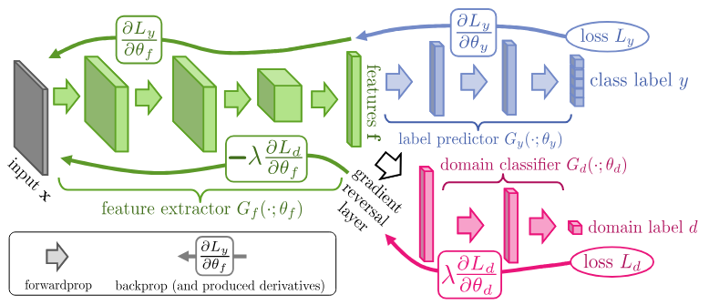
Figure 1: DANN architecture for domain-adversarial feature learning 1
—
1. Feature Extractor (\(G_f\))
This is the common trunk of the network.
It takes an input \(x\) and produces a feature vector:
\[z = G_f(x; \theta_f)\]Its parameters \(\theta_f\) are shared by both the task and domain branches and are trained with a dual, conflicting objective.
2. Label Predictor (\(G_y\))
The main classifier.
It takes the feature \(z\) and predicts the class label:
\[\hat{y} = G_y(z; \theta_y)\]It is trained only on the labeled source data to perform the primary task.
3. Domain Classifier (\(G_d\))
The adversarial component.
It takes the feature \(z\) and predicts the domain label:
\[\hat{d} = G_d(z; \theta_d), \quad d = 0 \text{ (source)}, \; d = 1 \text{ (target)}\]It is trained on both the source and target data to accurately distinguish the domains.
Adversarial Objective and Loss Function
The training process for DANN is a single-step optimization that simultaneously minimizes the task loss and plays the adversarial game to align features.
A. The Optimization Goal
The DANN optimization seeks to find the optimal parameters
\(\theta_f,\ \theta_y,\ \theta_d^{*}\)
that satisfy the following two competing objectives:
-
Task Loss Minimization:
The label predictor (\(G_y\)) and feature extractor (\(G_f\)) are optimized to minimize the error on the source domain labels. This ensures the model is discriminative for the classification task. -
Domain Confusion:
The domain classifier (\(G_d\)) is optimized to minimize its error (i.e., maximize its ability to distinguish the domains), while the feature extractor (\(G_f\)) is optimized to maximize the domain classifier’s error (i.e., make the domains indistinguishable). This forces the features to become domain-invariant.
B. The Total Loss Function
The final combined loss function \(E\) for the entire network is:
\(E(\theta_f, \theta_y, \theta_d) = L_y(\theta_f, \theta_y) - \lambda L_d(\theta_f, \theta_d)\) Where:
-
\(L_y\): The Task Loss (e.g., standard cross-entropy) computed only on the labeled source data. It is minimized: \(\theta_f, \theta_y \leftarrow \arg\min L_y\)
- \(L_d\): The Domain Loss (e.g., binary cross-entropy) computed on both source and target features.
- \(\theta_d\) is trained to minimize \(L_d\) (get better at domain classification).
- \(\theta_f\) is trained to maximize \(L_d\) (get worse at domain classification, confusing the discriminator).
- \(\lambda\): A positive hyperparameter that controls the trade-off between the two losses.
A common practice is to dynamically increase \(\lambda\) during training using a function like \(\lambda_p = \frac{2}{1 + e^{-\gamma p}} - 1\) where \(p\) is the training progress.
The optimization can be summarized as:
\[\theta_f^{*}, \theta_y^{*} = \arg\min_{\theta_f, \theta_y} E \quad \text{and} \quad \theta_d^{*} = \arg\min_{\theta_d} L_d\]This is equivalent to:
\[\theta_f^{*}, \theta_y^{*} = \arg\min_{\theta_f, \theta_y} \bigl( L_y + \lambda \cdot \text{Maximizing } L_d \bigr)\]Gradient Reversal Layer (GRL)
The most crucial component of DANN is the Gradient Reversal Layer (GRL), which enables the two conflicting objectives—minimizing \(L_y\) and maximizing \(L_d\) with respect to \(\theta_f\)—to be trained simultaneously using standard backpropagation.
The GRL is placed between the feature extractor \(G_f\) and the domain classifier \(G_d\).
The GRL operates as follows:
-
Forward Pass:
The GRL acts as an identity function, passing the feature vector \(z\) through unchanged: \(R_\lambda(z) = z\) -
Backward Pass (Backpropagation):
During backpropagation, the GRL multiplies the gradient flowing from the domain classifier by a negative scalar \(-\lambda\) before passing it to the feature extractor: \(\frac{\partial R_\lambda}{\partial z} = -\lambda I \quad \text{(where } I \text{ is the identity matrix)}\)
How the GRL Achieves Adversarial Training
-
For the Domain Classifier (\(\theta_d\)):
The parameters \(\theta_d\) are updated using the gradient of \(L_d\) to minimize \(L_d\).
The domain classifier receives the gradient before the sign reversal introduced by the GRL. -
For the Feature Extractor (\(\theta_f\)):
When the gradient flows back through the GRL to \(\theta_f\), its sign is flipped.
Since backpropagation performs gradient descent \(\theta \leftarrow \theta - \alpha \frac{\partial E}{\partial \theta},\) multiplying the gradient of \(L_d\) by \(-\lambda\) effectively converts the minimization of \(L_d\) into the maximization of \(L_d\) with respect to the shared parameters \(\theta_f\).
Conclusion:
While DANN acts as one of the first foundational papers in image-level UDA, the real-world autonomous vehicles need pixel-level labels or semantic segmentation. For example, DANN excels in identifying that a picture is of a dog, however, a useful model would need to identify that there is a dog in the center of the screen, crossing the road. The rest of the blog will explore how models can become spatially and structurally more aware, and therefore more useful for real-world application.
CyCADA: Cycle-Consistent Adversarial Domain Adaptation
CyCADA (Cycle-Consistent Adversarial Domain Adaptation) is a highly influential Unsupervised Domain Adaptation (UDA) method designed to address the challenges of domain shift in dense prediction tasks, primarily semantic segmentation. It advances beyond earlier approaches like DANN by introducing adaptation across two fundamental representation spaces: the pixel space and the feature space.
1. Core Methodology: Dual-Level Adaptation
The basic idea behind CyCADA is that to minimize the domain gap, you need to use consistent constraints at different levels of the network. The architecture simultaneously enforces three key properties during training:
- Pixel-Level Alignment: The appearance, or style, of the source domain (\(D\_S\)) is translated into the target domain’s style (\(D\_T\)). This reduces the low-level, high-frequency disparity (textures, lighting).
- Feature-Level Alignment: The high-level semantic features extracted from both the translated source images and the raw target images are statistically aligned, ensuring the representations are domain-invariant.
- Semantic Consistency: The fundamental content and structure (the ground truth mask) of the source image must remain unaltered after the style translation. This is crucial for maintaining label validity.
Essentially, what CyCADA achieves is using style transfer techniques, it transforms synthetic images to have the visual appearance of real-world data, while keeping their pixel labels intact. The model then learns from these realistic-looking images with guaranteed correct labels, and aligns features at a deeper level to ensure the translation preserves semantic meaning.
2. Architectural Components
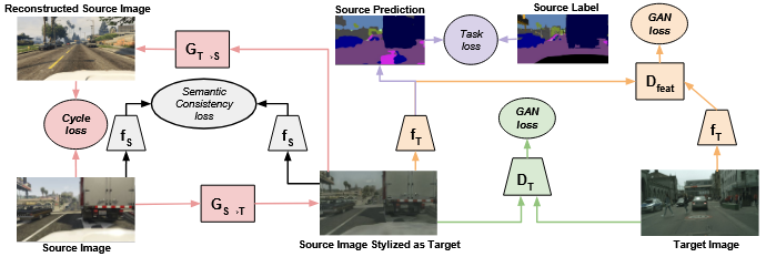
Figure 2: CyCADA architecture combining cycle-consistent image translation and feature-level adversarial learning for unsupervised domain adaptation 2
CyCADA integrates three specialized modules to achieve its objectives:
2.1. Cycle-Consistent Generative Adversarial Network (CycleGAN)
The pixel-level adaptation is implemented using a CycleGAN framework, which utilizes two generators (\(G_{S \to T}\) and \(G_{T \to S}\)) and corresponding discriminators (\(D_T\) and \(D_S\)). The core capability is to perform style transfer between the unpaired source and target datasets.
The generator \(G_{S \to T}\) is essential, as it produces the stylized source images \(x_s^{T} = G_{S \to T}(x_s),\) which retain the original labels \(y_s\) while adopting the target-domain style.
2.2. Semantic Segmentation Network
A standard Fully Convolutional Network (FCN), denoted as \(f\), serves as the backbone for the task. The feature extractor component of \(f\) is shared across both domains, while the classifier head is trained solely on the stylized source data.
2.3. Feature-Level Discriminator (\(D\_{feat}\))
This component is conceptually derived from DANN. \(D\_{feat}\) is attached to an intermediate feature map of the segmentation network \(f\). It is trained to distinguish between features originating from raw target images (\(x\_t\)) and features originating from stylized source images (\(x\_s^T\)).
3. Optimization Objective
The total loss function, \(L\_{total}\), is a composite objective comprising five distinct terms, weighted by hyperparameters \(\\lambda\):
\[L_{total} = L_{task} + \lambda_{cyc} L_{cyc} + \lambda_{sem} L_{sem} + \lambda_{GAN} L_{GAN} + \lambda_{feat} L_{feat}\]3.1. \(L\_{task}\) (Segmentation Loss)
This is the standard cross-entropy loss applied to the primary task on the labeled, stylized source images (\(x\_s^T\)):
\[L_{task} = L_{CE}\bigl(f(x_s^{T}), y_s\bigr)\]3.2. \(L\_{cyc}\) (Cycle-Consistency Loss)
A standard \(\\ell\_1\) loss minimizing the reconstruction error, ensuring the style transfer does not destroy image structure:
\[L_{cyc} = \lVert G_{T \to S}\bigl(G_{S \to T}(x_s)\bigr) - x_s \rVert_1 + \lVert G_{S \to T}\bigl(G_{T \to S}(x_t)\bigr) - x_t \rVert_1\]3.3. \(L\_{sem}\) (Semantic Consistency Loss)
This novel term is critical for semantic segmentation. It minimizes the distance between the segmentation predictions generated by \(f\) for the original source image \(x\_s\) and the stylized source image \(x\_s^T\). This enforces that the domain translation preserves high-level semantics:
\[L_{sem} = L_{CE}\bigl(f(x_s), f(x_s^{T})\bigr)\]3.4. \(L\_{feat}\) (Feature Adversarial Loss)
The adversarial loss driving the domain alignment of intermediate features. The feature extractor of \(f\) is trained to maximize this loss (confuse \(D\_{feat}\)), while \(D\_{feat}\) is trained to minimize it:
\[L_{feat} = \min_{f} \max_{D_{feat}} \mathbb{E}_{x_s \in D_S} \bigl[ \log D_{feat}\bigl(f(G_{S \to T}(x_s))\bigr) \bigr] + \mathbb{E}_{x_t \in D_T} \bigl[ \log \bigl(1 - D_{feat}(f(x_t))\bigr) \bigr]\]By combining these constraints, CyCADA achieved stability and performance gains that were unattainable with earlier global feature alignment methods, marking a significant step toward robust domain adaptation for dense prediction.
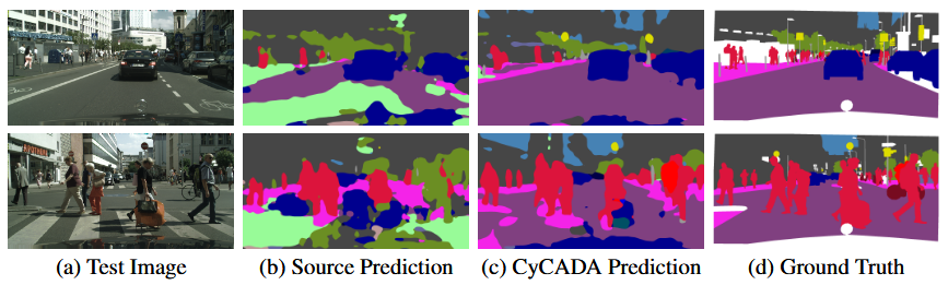
Figure 3: Qualitative comparison of source-only and CyCADA segmentation predictions on Cityscapes 2
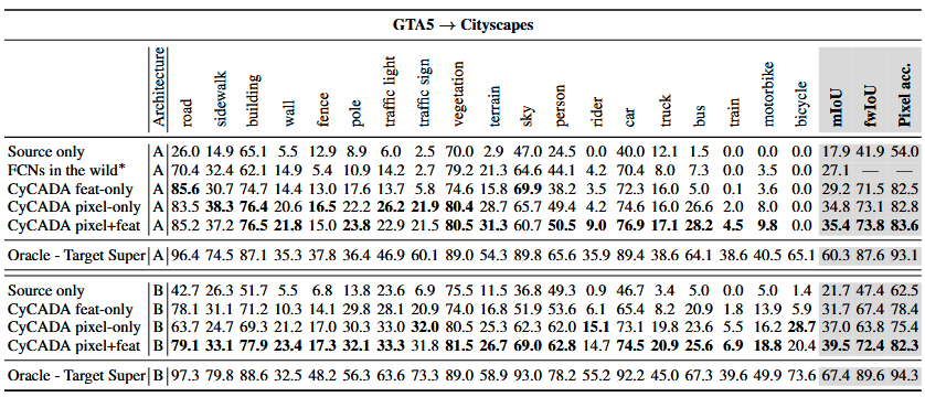
Table 1: Per-class IoU, mean IoU, and pixel accuracy for adaptation from GTA5 to Cityscapes. CyCADA significantly outperforms source-only baselines across architectures 2
Conclusion:
While the performance of CyCADA receives a 39.5 mIoU, the computation done to modify the source domain to the target domain’s statistics before being classified is an image-to-image transformation. Recognizing these limitations, subsequent research shifted focus from modifying the input features to regularizing the model’s output. This evolution led to ADVENT, a method that eschews style transfer entirely and instead leverages the adversarial principle to enforce confidence by minimizing prediction entropy in the target domain’s output space.
ADVENT: Adversarial Entropy Minimization for Domain Adaptation
ADVENT is based around a simple, yet insightful observation: when models are confident, they work well. On synthetic data, models tend to make confident predictions, whereas on real-world data, predictions tend to become fuzzy. So instead of transforming images or aligning internal features, ADVENT directly forces the model to be confident on real-world data.
More formally, ADVENT (Adversarial Entropy Minimization) is an Unsupervised Domain Adaptation (UDA) technique specifically tailored for semantic segmentation that approaches the domain shift problem by focusing on the output space of the model rather than intermediate feature statistics. Unlike methods that modify input images (like CyCADA) or align internal feature representations (like DANN), ADVENT uses an adversarial discriminator that can spot uncertain predictions and leverages the principle of entropy minimization to enforce confidence and stability in the target domain predictions.
1. Theoretical Foundation: Entropy as a Domain Gap Metric
As mentioned prior, ADVENT is founded on the observation that predictions made on the source domain (\(D\_S\)) are generally low-entropy (high confidence), whereas predictions on the target domain (\(D\_T\)) often exhibit high-entropy (high uncertainty) due to domain shift.
1.1. Entropy Definition
For a prediction map \(P(y \mid x_t)\) generated by the segmentation network \(f\) for a target image \(x_t\), the local entropy \(H_{i,j}\) at pixel \((i,j)\) is defined as:
\[H(P(y \mid x_t)) = H_{i,j} = -\sum_{c=1}^{K} p_{i,j}^{c} \log p_{i,j}^{c}\]where \(p_{i,j}^{c}\) is the predicted probability for class \(c\) at pixel \((i,j)\), and \(K\) is the total number of classes.
1.2. The Objective
The core objective of ADVENT is to train the segmentation network \(f\) to produce output probability maps for \(D\_T\) that possess low entropy, effectively minimizing the uncertainty induced by the domain gap. Direct minimization of entropy can lead to trivial local minima; therefore, ADVENT introduces an adversarial mechanism to implicitly enforce this constraint.
2. Adversarial Formulation
ADVENT utilizes an adversarial setup to implicitly enforce entropy minimization by aligning the distribution of uncertainty across domains.
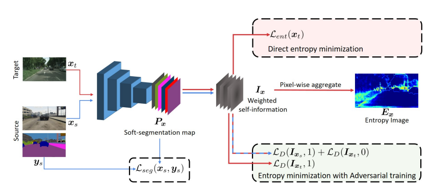
Figure 4: ADVENT architecture for unsupervised domain adaptation 3
2.1. Architectural Components
- Semantic Segmentation Network (\(f\)): A standard FCN or DeepLab network that performs the pixel-level classification. Its parameters \(\\theta\_f\) are the primary target of optimization.
- Domain Discriminator (\(D\)): A convolutional network trained to distinguish between the uncertainty profiles of \(D\_S\) and \(D\_T\).
2.2. The Input to the Discriminator
Crucially, the discriminator \(D\) does not take the raw feature map as input. Instead, it takes the output probability map \(P(y \mid x)\) from the segmentation network \(f\). Specifically, it often uses the weighted self-information map
\[I(x) = P(y \mid x) \cdot H\bigl(P(y \mid x)\bigr),\]which provides a structured representation that emphasizes regions of high uncertainty for the discriminator.
2.3. The Adversarial Game
The optimization is formulated as a minimax game:
- Discriminator (\(D\)) Goal: The discriminator parameters \(\\theta\_D\) are optimized to minimize the Binary Cross-Entropy (BCE) loss when correctly classifying the source output (assigned label 0) versus the target output (assigned label 1). This forces \(D\) to explicitly model the uncertainty difference between the two domains.
- Segmentation Network (\(f\)) Goal: The network parameters \(\\theta\_f\) are trained to maximize the discriminator loss for the target output. By maximizing \(D\)’s confusion, \(f\) is forced to generate target outputs that mimic the characteristics of source outputs (i.e., low entropy).
2.4. Total Optimization Loss
The total loss \(L\) used to train the segmentation network \(f\) is a combination of the task-specific supervised loss on \(D_S\) and the adversarial loss on \(D_T\):
\[L(\theta_f, \theta_D) = L_{CE}(\theta_f; D_S) + \lambda_{adv} L_{adv}(\theta_f; D_T)\]Where:
-
\(L_{CE}(\theta_f; D_S)\): The standard cross-entropy task loss calculated only on the labeled source domain.
-
\(L_{adv}(\theta_f; D_T)\): The adversarial loss calculated on the unlabeled target domain. This term guides \(\theta_f\) to align the output entropy.
-
\(\lambda_{adv}\): A hyperparameter that controls the influence of the adversarial regularization.
This iterative optimization process results in a segmentation network whose predictions on the target domain are structurally confident and robust against domain shift.
Note that for some datasets with significantly different layouts/viewpoints, ADVENT can lead to poor inference decisions, specifically for rare classes. The researchers utilize a class-ratio prior to encourage the presence of all classes, as to not ignore rare classes. They choose to use a value of 0.5, right in between having no prior and enforcing the exact class-ratio prior. DAFormer expands on this imbalance in the later section, tackling it with RCS.
3. Advantages of Output-Space Adaptation
ADVENT’s focus on the output space provides several distinct advantages over traditional feature-level adversarial methods:
- Enhanced Stability: Aligning the output probability distribution, which is intrinsically lower dimensional than intermediate feature maps, leads to a more stable adversarial training process.
- Direct Task Correlation: Regularizing the output directly enforces a desirable property (confidence/low uncertainty) that is highly correlated with strong final task performance, offering a more direct path to adaptation success.
- Computational Efficiency: The method avoids the computational overhead associated with training and running image-to-image translation models, as required by approaches like CyCADA.
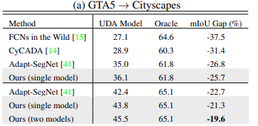
Table 2: Comparison of mean IoU and oracle performance for unsupervised domain adaptation from GTA5 to Cityscapes. ADVENT improves segmentation performance over prior methods 3
Conclusion:
Not only does ADVENT improve on CyCADA with an mIoU of 45.5, ADVENT is a lot less computationally demanding. There is no need to perform transformations mapping one image to the test domain, but instead can allow training solely on the entropy loss. However, ADVENT still uses adversarial training which introduces optimization instability, due to balancing two opposite loss functions. In addition, the architectural backbone is still CNNs. Through exploring a new foundation with the transformer architecture model, this blog will now focus on the DAFormer model.
DAFormer: Domain-Adaptive Transformer
DAFormer (Domain-Adaptive Transformer) represents a paradigm shift in Unsupervised Domain Adaptation (UDA) for semantic segmentation, moving away from conventional Convolutional Neural Network (CNN) backbones and feature alignment tricks toward leveraging the inherent domain generalization capabilities of the Transformer architecture. The work introduces architectural enhancements and novel training strategies that collectively achieve a substantial improvement in performance on benchmarks like GTA5 → Cityscapes.
1. Architectural Foundation: The MiT Encoder
DAFormer is built upon a high-performance segmentation architecture, replacing the typical ResNet/VGG backbone with the Mix Transformer (MiT) encoder.
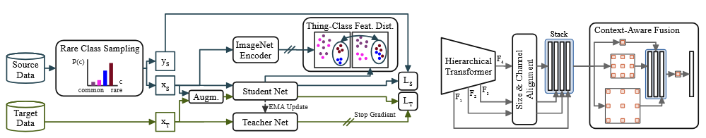
Figure 5: DAFormer architecture for domain-adaptive semantic segmentation using transformer-based feature alignment and context-aware fusion 4
1.1. Mix Transformer (MiT)
The MiT encoder, used in the SegFormer architecture, naturally benefits UDA due to its ability to capture global context via self-attention mechanisms. Unlike CNNs, which have local receptive fields, Transformers can model long-range dependencies across the entire input image. This global context is crucial because the semantic meaning of pixels in the target domain often depends heavily on distant elements in the scene (e.g., classifying a small road sign relies on understanding the surrounding road and sky). This global view makes the feature representation inherently more robust to local texture and style shifts common in domain gaps, allowing it to make more accurate predictions on unlabeled images in the target domain.
1.2. Context-Aware Feature Fusion
The decoder utilizes a lightweight, context-aware mechanism that effectively fuses multi-scale features generated by the MiT encoder. This fusion is essential for recovering fine details necessary for accurate pixel-level segmentation boundaries.
2. Novel Training Strategies
The architectural shift is complemented by three highly effective training strategies designed to maximize the domain robustness of the Transformer backbone, particularly for challenging classes.
2.1. Rare Class Sampling (RCS)
The unsupervised adaptation process often suffers from a class-imbalance bias. Common classes (e.g., road, building, sky) are easily pseudo-labeled, leading to high confidence and strong alignment, while rare classes (e.g., traffic sign, bicycle, train) are poorly adapted.
RCS addresses this issue by modifying the sampling distribution of the labeled source domain \(D_S\) used during adaptation. Images containing rare classes are sampled more frequently than under a uniform distribution. This ensures that both the adversarial and task losses receive sufficient contribution from minority classes, preventing them from being ignored during feature alignment.
Let \(N_c\) denote the number of pixels belonging to class \(c\) in the source dataset. The sampling probability for image \(i\), denoted by \(P(i)\), is computed based on the class frequencies present in the image:
\[P(i) = \frac{\sum_{c \in I_i} f_c^{-1}}{\sum_c f_c^{-1}}, \qquad f_c = \log(\tau + N_c)\]where \(I_i\) is the set of classes present in image \(i\), and \(\tau \ge 1\) is a hyperparameter that moderates the inverse frequency. This procedure effectively prioritizes images containing underrepresented classes, ensuring more robust feature learning across all categories.
2.2. Thing-Class ImageNet Feature Distance (T-CIFD)
Transformers are typically initialized with weights pre-trained on large-scale classification datasets such as ImageNet. This pre-training is crucial for learning rich and transferable object representations for “thing” classes (objects with countable instances such as people or cars). However, domain adaptation can cause the model to drift away from these pretrained features.
T-CIFD introduces a regularization term that preserves feature transferability for thing classes by minimizing the feature distance between the source-domain and target-domain representations, while applying this constraint only to thing classes.
\[L_{\text{T-CIFD}} = \frac{1}{|C_{\text{thing}}|} \sum_{c \in C_{\text{thing}}} \left\| \mu(F_c^{\text{source}}) - \mu(F_c^{\text{target}}) \right\|_2^2\]where \(C_{\text{thing}}\) is the set of thing classes, and \(\mu(F_c)\) denotes the mean feature vector of all pixels belonging to class \(c\). This constraint prevents the feature extractor from drastically altering learned object representations, while still allowing “stuff” classes (e.g., road, sky) to adapt flexibly to the target domain.
2.3. Learning Rate Warmup
Due to the sensitivity of Transformer models to initial training instability, DAFormer uses a simple but effective linear learning rate warmup at the beginning of the adaptation phase. This stabilizes the training process and is shown to significantly contribute to the final performance gain.
By combining the powerful, context-aware MiT backbone with strategic training methods like RCS and T-CIFD, DAFormer achieved state-of-the-art performance, demonstrating that architecture and targeted regularization are more impactful than simple GAN-based alignment in modern UDA for semantic segmentation.
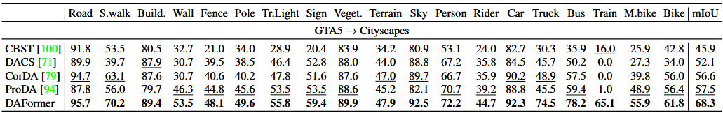
Table 3: Per-class IoU and mean IoU for unsupervised domain adaptation from GTA5 to Cityscapes, comparing DAFormer with prior methods 4
With an mIoU of 68.3, DAFormer beats both CyCADA and advent with its transformer based architecture. As the foundational transformer based architecture model, it paved the way for future papers to build off of it. In fact, the DAFormer team also published Hierarchical Domain-invariant Representation Alignment (HDRA) which performed with 73.8 mIoU.
Performance Comparison & Conclusion
The progression from CyCADA to DAFormer shows dramatic performance improvements in domain adaptation research. Testing on the standard GTA5 → Cityscapes benchmark reveals just how far the field has advanced:
| Method | Backbone | Architecture Type | mIoU (%) |
|---|---|---|---|
| CyCADA | ResNet-101 | CNN + GAN | 39.5 |
| Advent | ResNet-101 | CNN + Entropy | 45.5 |
| DAFormer | MiT-B5 | Transformer | 68.3 |
CyCADA’s solution in bridging the domain gap was on the pixel-level foundation. It transformed GTA5 images to look like real photographs through style transfer, then trained on these “realistic” synthetic images. Thus by reducing low-level appearance differences (color, texture, lighting), CyCADA makes it easier for the CNN to recognize familiar patterns. However, the method is computationally expensive, requiring training complex GAN-based image translation networks. And more critically, perfect pixel-level alignment is near impossible. Real-world images have variations that can’t be captured by translating synthetic data. The CNN backbone also struggles to leverage global context, limiting how well features can align.
ADVENT took a different approach through focusing on making the model’s predictions confident. By working directly in the output space and minimizing entropy, ADVENT achieved better results with far less computational overhead since it avoids the computational burden of image translation while addressing the core problem: uncertain predictions on target data. But ADVENT still uses a CNN backbone (ResNet-101) that relies on local receptive fields. So when low-level textures differ significantly between domains, CNNs can struggle to make confident predictions no matter how much the entropy loss tries to force confidence.
This is where DAFormer introduces a major shift in the approach to architecture. By switching to a Transformer backbone, DAFormer gains the ability to capture global context through self-attention, making it naturally more robust to local appearance differences. The self-attention mechanism essentially lets the model consider the entire image when making predictions, which allows it to use spatial and structural relationships to make consistent predictions across domains. And through smart training strategies such as RCS, which ensures rare classes aren’t ignored during adaptation, it further increases the model’s ability in recognizing objects between images in different domains. This paradigm shift explains the jump from 45.4% to 68.3% in mIoU.
As these unsupervised domain adaptation models drastically increase in performance with new architectures each year, it’s only a matter of time before we see these systems deployed on real roads. When CyCADA was first published in 2017, the state of the art model that trained on the target domain (not the source domain like our UDA models), only had 67.4 mIoU. Compare that to HDRA’s 2023 result training on the source domain at 73.8 mIoU.
In order for vehicles to achieve true autonomy, they need rigorous training and many test runs in the real-world. However, with improved UDA models, this real-life test time can be drastically reduced. With these models, the models can be trained to align features between Day/Night, Clear/Foggy, and even US/India roads! While these different domains are very different, improvement in the models can lead to a future where the Tesla trained on the GTA5 dataset set in America can be deployed to China with minimal modifications.
References
[1] Ganin, Y., et al. “Domain-adversarial training of neural networks.” JMLR 2016.
[2] Hoffman, J., et al. “CyCADA: Cycle-Consistent Adversarial Domain Adaptation.” ICML 2018.
[3] Vu, T., et al. “ADVENT: Adversarial Entropy Minimization for Domain Adaptation in Semantic Segmentation.” CVPR 2019.
[4] Hoyer, L., et al. “DAFormer: Improving Network Architectures and Training Strategies for Domain-Adaptive Semantic Segmentation.” CVPR 2022.