Evolution of Human Pose Estimation - From Deep Regression to YOLO-Pose
Human pose estimation is a fundamental problem in computer vision that focuses on localizing and identifying key body joints, such as elbows, knees, wrists, and shoulders of a person through images or video. By predicting these keypoints or predefined body landmarks, models can infer a structured, skeleton-like representation of the human body, which enables further exploration into understanding human posture, motion, and interactions with the environment. As such, this field is a crucial area of research that is used in various real-world applications like action recognition or healthcare. In this project, we study a variety of different deep learning approaches to 2D human pose estimation, beginning first with early end-to-end regression models and progressing towards more structured and context-aware architectures. In particular, we delve deeper into how modeling choices around global context, spatial precision, and body structure influence pose estimation performances.
Table of Contents
- Introduction
- Background & Fundamentals
- Stacked Hourglass Networks
- Adversarial Learning of Structure-Aware Fully Convolutional Networks
- YOLO-Pose: Real-Time Multi-Person Pose Estimation
- Conclusion
- References
Introduction
Project Overview
Human pose estimation is a fundamental problem in computer vision that focuses on localizing and identifying key body joints, such as elbows, knees, wrists, and shoulders of a person through images or video. By predicting these keypoints or predefined body landmarks, models can infer a structured, skeleton-like representation of the human body, which enables further exploration into understanding human posture, motion, and interactions with the environment. As such, this field is a crucial area of research that is used in various real-world applications like action recognition or healthcare. In this project, we study a variety of different deep learning approaches to 2D human pose estimation, beginning first with early end-to-end regression models and progressing towards more structured and context-aware architectures. In particular, we delve deeper into how modeling choices around global context, spatial precision, and body structure influence pose estimation performances.
Problem Statement
Accurately estimating human pose is challenging due to a few inherent factors. Human bodies are highly articulated, which can lead to large variations in joint configurations across different poses. Additionally, occlusions and cluttered backgrounds can further complicate joint localization, especially for those smaller or ambiguous joints such as wrists and ankles. Pose estimation also requires pixel-level precision, since correct joint placement often depends on understanding the overall global configuration of the entire body rather than just the local image cues themselves.
Paper Scope
This paper focuses on single-person and multi-person 2D human pose estimation using deep learning methods. We will begin first by introducing DeepPose, one of the earliest and foundational deep learning approaches to pose estimation, which framed the task as a direct joint regression problem. We then discuss later models, such as Stacked Hour Glass Networks, Adversarial Structure-Aware approaches, and YOLO-based pose estimators. Our analysis will focus on architectural design choices, dataset usage, evaluation metrics, and how each method and their approaches improved structural reasoning and robustness in this field.
Use Cases
Human pose estimation is widely used across various domains. For example, in sports analytics, pose estimation helps enable motion analysis and performance feedback. In healthcare, it supports everything from physical therapy monitoring to fall detection. In addition, with recent developments in animation, robotics, and gaming, pose estimation plays an important role as it allows real-world human actions to be transferred to digital characters and experiences. With such varied applications, human pose models continue to evolve in both accuracy and robustness to challenging visual conditions.
Background & Fundamentals
DeepPose
First we will take a look at DeepPose, which was introduced by Alexander Toshev and Christian Szegedy from Google. It was one of the first works to apply deep convolutional neural networks to human pose estimation, and instead of relying on part-based detectors or graphical models, DeepPose formulated pose estimation as a direct regression problem. Specifically, a single CNN predicted the 2D coordinates of all the body joints simultaneously from the full input image.
\[L = \sum_{i=1}^{k} \|\hat{y}_i - y_i\|_2^2\]Fig 1. Joint regression loss: K is the number of body joints, $y_i$ is the ground truth 2D location of joint i, and $\hat{y}_i$ is the predicted joint location.
The model uses an AlexNet-style architecture to produce an initial course prediction of joint location, and then to improve accuracy, it adds a coarse-to-fine cascade, where subsequent stages will crop local image regions around each predicted joint to refine their position in an iterative process. This approach allows the network to progressively increase spatial precision, while still maintaining its awareness of the global body layout as a whole.
DeepPose demonstrated that end-to-end CNN regression is viable for pose estimation and it achieved state-of-the-art results at the time on benchmarks such as FLIC and LSP. Its primary areas of improved performance included the previously discussed difficult wrist and elbow joints. As such, DeepPose established itself as a foundational paradigm that many later methods would refine and extend.
While revolutionary, DeepPose did have its limitations. Specifically, direct coordinate regressions are known to struggle with multi-modal outputs, and also lack explicit spatial structure, which in turn makes it difficult to enforce various anatomical constraints or recover from large initial errors. These shortcomings are what motivated later approaches to adopt heatmap-based representations and repeated multi-scale reasoning which we will later discuss.
Datasets
In terms of datasets, human pose estimation models are commonly evaluated on a small set of standard benchmark datasets. Early deep learning approaches like DeepPose or Stacked Hourglass Networks mainly used the FLIC and MPII Human Pose datasets. FLIC focuses on upper-body joints from sources like movie scenes, and it serves as an early benchmark for joint localization accuracy. MPII provides full-body annotations across a wide range of everyday activities and poses, and is more comprehensive and adopted as a benchmark for single-person pose estimation.
Some additional datasets worth noting as they help evaluate the robustness of the model as they include more complex conditions. For instance, the Leeds Sports Pose (LSP) dataset has extreme athletic poses, and is commonly used for performance tests on highly articulated joints. More recent methods such as the multi-person approach with YOLO-Pose, use MS COCO Keypoints dataset, which includes crowded scenes and multiple interacting people. Overall, these datasets reflect the range of possible poses, and also the increasing complexity that modern models hope to tackle.
Challenges
Human pose estimation presents several recurring challenges that are faced across different architectures and the datasets that they are evaluated on. Occlusion, which in this case is partiall or fully hidden joints, is one of the biggest issues. Additionally, there are cases of ambiguity when image evidence might be not be enough to distinguish between symmetric limbs or overlapping body parts. Scale variation and viewpoint changes, which are prevalent in many areas of computer vision research, add additional complications to joint localization as well. All in all, balancing global structural consistency with the pixel-level accuracy needed presents an interesting challenge for different models as they consider the tradeoffs that ultimately lead to different architectural design choices.
Evaluation
Pose estimation models are commonly evaluated using metrics such as Percentage of Correct Keypoints (PCK) or PCKh, which measures whether or not the predicted joints are within the normalized distance threshold of the ground-truth location. These metrics focus on both the localization accuracy, and how well the model is to extend across various joints. Evaluations are usually reported per joint and averaged across the dataset, which allows additional insights on the more difficult joints and more general overviews.
Stacked Hourglass Networks for Human Pose Estimation
One of the main problems that DeepPose and other human pose estimation models faced was that joint predictions must be really precise (down to the pixel), but their correct placement heavily depends on the global body configuration. When looking at a local section of an image, where to place the joint is often ambiguous (especially under occlusion). The Stacked Hourglass Networks for Human Pose Estimation paper by Alejandro Newell, Kaiyu Yang, and Jia Deng from the University of Michigan argues that strong pose estimation requires repeated reasoning across scales, not just a single pass through a multi-scale network like previous models.
The Architecture
The central component of the model is the hourglass module, named after its symmetric structure. Each hourglass performs bottom-up processing through convolution and max pooling, which gradually reduces the spatial resolution until it reaches a very small representation (sometimes as small as 4×4). At this scale, the features have a global receptive field and can encode relationships between really distant joints (such as the relative positions of hips, knees, and shoulders).
Then, the network performs a top-down processing, which uses nearest-neighbor upsampling to recover the spatial resolution. This is similar to a U-Net architecture. Skip connections are added to merge features from corresponding resolutions both on the way down and up, which enables the model to preserve really precise spatial detail while still incorporating global context. The importance of the module is its symmetrical design, since the hourglass from earlier fully convolutional or encoder–decoder designs emphasize bottom-up computation more.
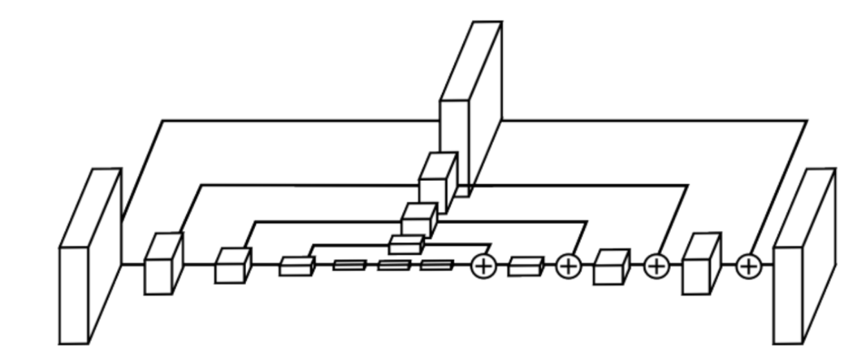
Fig 2. The stacked hourglass module architecture.
The model then stacks these multiple hourglass modules end-to-end. Each hourglass module takes the features and predictions of the previous stage as input and produces a new set of pose predictions. This is how the network is able to iteratively refine its pose estimates.
The paper discusses that most pose errors come from structural inconsistencies. This includes things like assigning a wrist to the incorrect arm or confusing right and left limbs. This is really challenging to fix with just local refinement, but by continuing to perform bottom-up and top-down inference, the later hourglass modules can refine their earlier predictions with a better understanding of the global pose.
Supervision and Loss Function The model uses dense supervision by training on ground-truth heatmaps, where for each joint k, a ground-truth heatmap H*k is created that is represented as a 2D Gaussian distribution which is centered at the true joint location l_k.
\[H^*_{k}(x, y) = \exp\left( - \frac{\|(x, y)-l_k\|^2}{2\sigma^2} \right)\]They use the mean squared error of the predicted and ground-truth heatmaps as their loss function. One key design choice to point out is that they used intermediate supervision, which means this loss is applied after every hourglass module. This forces each stage of training to check itself and improve performance and convergence speed.
Implementation details
The paper also discusses the use of residual models throughout the architecture. They avoid filters over 3x3 to ensure that the parameter counts stay manageable. The input image is resized to 256x256, and the prediction output size is 64x64. The final predictions are further refined by a small (less than a pixel) offset based on the neighboring heatmap activations.
They utilized data augmentation during their training including rotation and scaling, but they avoided using translation. This is mainly due to the fact that the model is trained to predict the pose of the centered person in the image, which simplifies the problem. This means that the model is not able to do multi-person reasoning.
Results
The model at the time of publication achieved state-of-the-art performance on both FLIC and MPII benchmarks. Gains are especially large for difficult joints such as wrists, elbows, knees, and ankles, where global context is critical. Ablation experiments show that stacking hourglasses improves accuracy even when total model capacity is held constant, and that intermediate supervision provides additional gains.
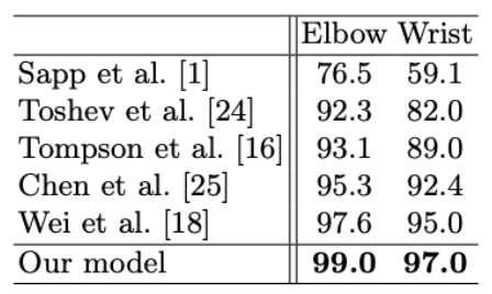
Fig 3. PCKh results on the FLIC benchmark dataset.
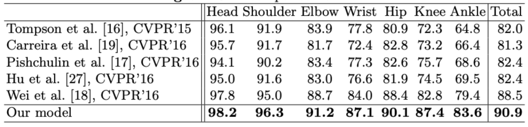
Fig 4. PCKh results on the MPII Human Pose benchmark dataset.
Conclusion
The equations in Stacked Hourglass Networks are intentionally simple but what makes them incredibly powerful is the architectural design. By repeatedly applying the same prediction mechanism and using intermediate supervision at every stage, the network learns to correct its own structural mistakes. This work was really influential in later pose estimation models and established stacked, heatmap-based architectures with intermediate supervision as a standard approach for human pose estimation.
Adversarial Learning of Structure-Aware Fully Convolutional Networks for Landmark Localization
In 2019, a new structure-aware approach to pose estimation was introduced in Adversarial Learning of Structure-Aware Fully Convolutional Networks for Landmark Localization. Researchers Yu Chen, Chunhua Shen, Hao Chen, Xiu-Shen Wei, Lingqiao Liu, and Jian Yang found inspiration in human vision, which is capable of both inferring potential poses and excluding implausible ones (even in the presence of severe occlusions). Prior solutions, such as stacked hourglass, imposed no constraints on potentially producing biologically implausible pose predictions and continue to struggle to overcome common challenges in pose estimation such as heavy occlusions and background clutter (see comparison below). This paper proposes a solution to integrate the concept of geometric constraints into pose estimation by utilizing Generative Adversarial Networks (GANs).
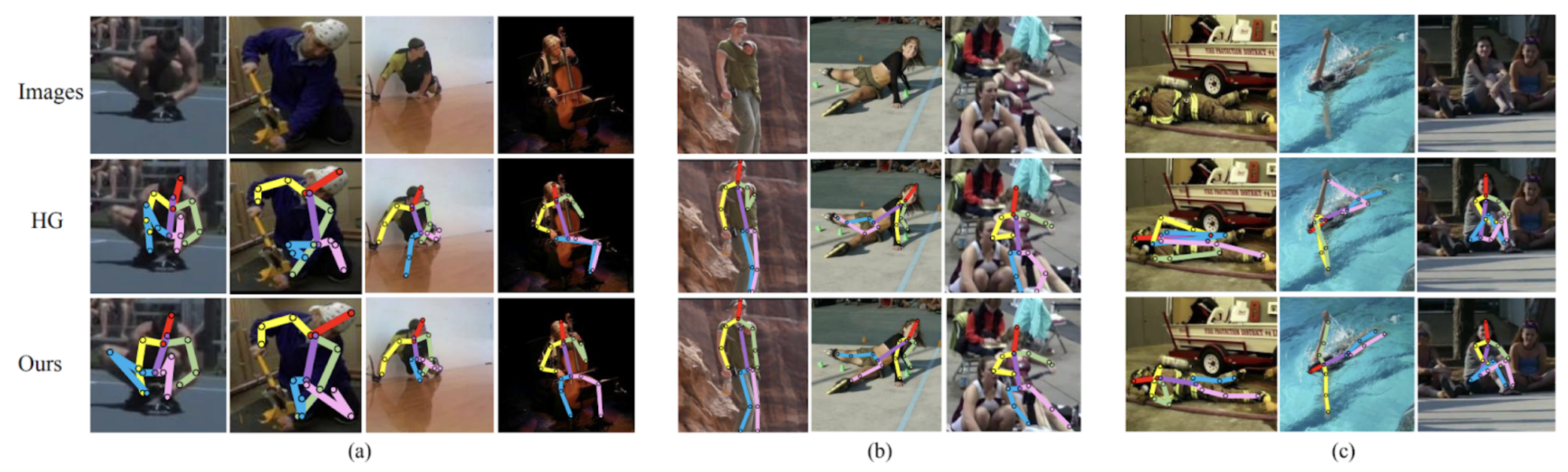
Fig 5. Prediction samples on the MPII set comparing stacked hourglass (HG) and adversarial learning (Ours).
The Architecture
A GAN sets up two networks as competitors in a zero-sum game: a generator G and a discriminator P. The GAN described in this paper encourages P to classify the plausibility of a pose configuration and G to generate pose heatmaps aimed to fool the discriminator. The authors additionally made other minor architectural changes (e.g. designing stacked multi-task networks) that achieved improved results for 2D pose estimation. The discriminator learns the structure of body joints implicitly through the following designs of the generator and discriminator.
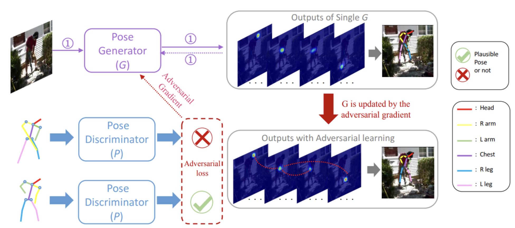
Fig 5. Structure-Aware Adversarial Training Model
Generative Network
The fully convolutional generative network implements the Stacked Hourglass architecture previously discussed to combine local joint features with global body context, ensuring neurons maintain large receptive fields. Like stacked hourglass, the image is processed using a convolution, residual bloc, and max pooling. The network then includes multiple stacking modules where pose heatmaps (body part locations) and occlusion heatmaps (hidden parts) are jointly predicted to calculate the intermediate losses. Additionally, the network can access previous estimates and features through the stacked modules, enabling the system to re-evaluate the joint predictions of poses and occlusions at any latter stage. Note, this paper discusses both 2D and 3D pose estimation; however, we will be focusing on 2D pose estimation in this discussion. In each block, 1 x 1 convolutions with residual connections reduce the number of feature maps down to the number of body parts then obtain the final predicted heatmaps. The resulting multi-task generative network is the baseline model in the paper’s framework whose goal is to learn a function 𝒢 that can project an image x to both the corresponding pose heatmaps y and the occlusion heatmaps z. The direct goal of 𝒢 is to minimize the Mean Squared Error between the predicted and ground-truth heatmaps to align spatial accuracy.
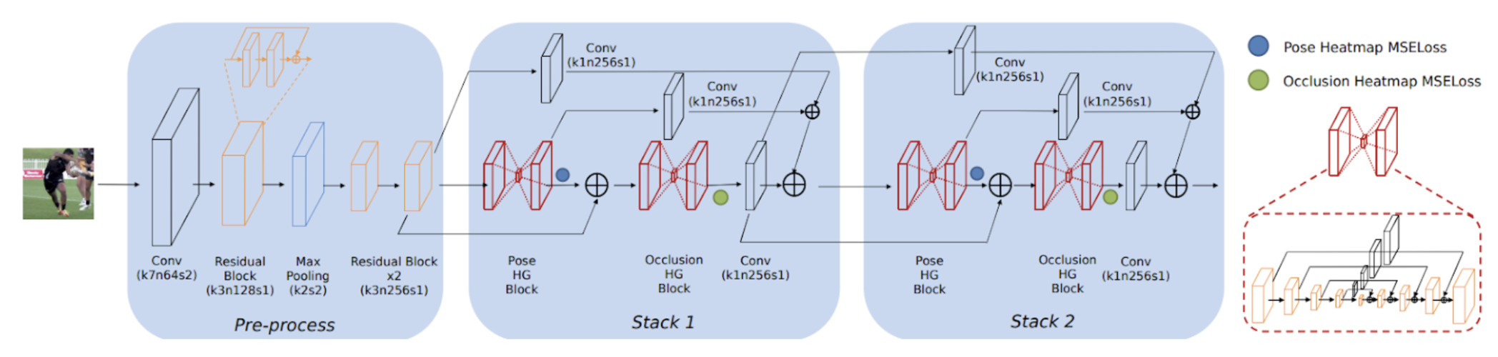
Fig 6. Generative Network G.
Discriminative Network
The pose discriminator employs an encoder-decoder architecture with skip connections to utilize the pose and occlusion heatmaps from the generator to predict whether each provided pose is physically reasonable. Both low-level details (local patches) and high-level context (global relationships) are crucial for judging pose plausibility. Skip connections between parallel layers help integrate local and global information. The discriminators additionally consider the original RGB image to ensure the model exclusively matches poses to the current image subject to avoid any poses that may potentially be plausible for another image but incorrect for the specific image subject. To enforce these constraints onto the generator, the design treats the GAN as a conditional GAN (cGAN) as P aims to maximize the objective function that classifies physically plausible poses as “real”.
The auxiliary discriminator, or confidence discriminator, is a specialized discriminator aimed to eliminate occlusion struggles using Gaussian centering by discriminating high-confidence predictions. The confidence discriminator heavily relies on the surrounding structure of an occlusion.
Adversarial Training
The generator G generates poses and occlusion information via heatmaps given to the discriminator. It is a fully convolutional neural network trained in an adversarial manner to deceive the discriminator. Following the standard implementation of a GAN, The discriminator P is designed to distinguish between real and fake poses and is trained to learn geometrically implausible poses as priors. The implicit logic is as follows: “G can “deceive” P => successfully learned priors” (explicitly learning keypoint constraints is difficult, motivating the implicit approach of the GAN). The paper aims to take priors into account by learning body joint distribution. The auxiliary discriminator also plays a specialized role but more or less follows the design of a standard adversarial minimax game.
Loss & Objective Functions
Generative Network Loss
Given a training set {xi, yi, zi}Mi=1, for M training images, the loss function is the following:
\[\mathcal{L}_G(\Theta) = \frac{1}{2MN} \sum_{n=1}^{N} \sum_{i=1}^{M} \left( \|\boldsymbol{y}^i - \hat{\boldsymbol{y}}_n^i\|^2 + \|\boldsymbol{z}^i - \hat{\boldsymbol{z}}_n^i\|^2 \right)\]Discriminitive Network Loss
Given the generator outputs G(x), the ground truth pose and occlusion heatmaps, and the ground truth label for the pose discriminator, the loss function is the following:
\[\mathcal{L}_P(G, P) = \mathbb{E}[\log P(\boldsymbol{y}, \boldsymbol{z}, \boldsymbol{x})] + \mathbb{E}[\log(1 - |P(G(\boldsymbol{x}), \boldsymbol{x}) - \boldsymbol{p}_{\text{fake}}|)]\]Confidence Discriminator Network Loss
Given Cfake is the ground truth confidence level, the loss function is the following:
\[\mathcal{L}_C(G, C) = \mathbb{E}[\log C(\boldsymbol{y}, \boldsymbol{z})] + \mathbb{E}[\log(1 - |C(G(\boldsymbol{x})) - \boldsymbol{c}_{\text{fake}}|)]\]Adversarial Objective
Given the hyperparameters and and the calculated losses, the final objective function is:
\[\arg \min_G \max_{P,C} \mathcal{L}_G(\Theta) + \alpha \mathcal{L}_C(G, C) + \beta \mathcal{L}_P(G, P)\]Training
Training the adversarial network follows this algorithm:
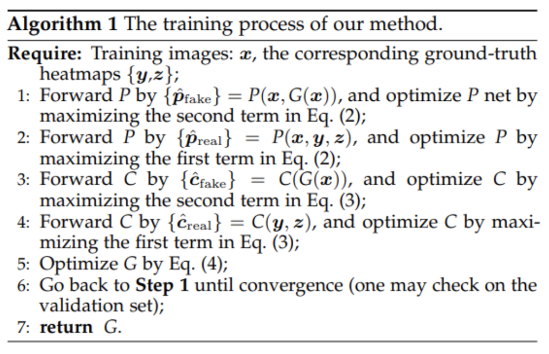
Fig 7. Adversarial training algorithm.
The algorithm iteratively learns the generator G, discriminator P, and confidence discriminator C. For both discriminators, each i-th fake label t is set to 1 if the normalized distance di between the prediction and ground truth is less than a threshold or , and 0 otherwise. These initializations for the discriminators coerce G into generating biologically plausible poses with high-confidence. The algorithm then iteratively learns the generator G, discriminator P, and confidence discriminator C with respect to each loss function and the combined objective function.
Results
Numerically, the proposed architecture in this paper did make improvements upon the state-of-the-art competitors at the time. The paper evaluated the 2D Human Pose estimation on Leeds Sports Poses (LPS), MPII Human Pose, and MSCOCO Keypoints dataset. Accuracy is evaluated on percentage of correct keypoints (PCK). For the LSP dataset, this method achieved the second-best performance with a 2.4% improvement over previous methods on average. For the MPII Human Pose dataset, this method achieves the best PCK with a score of 91.9% with notable improvements on difficult joints such as wrists and ankles.
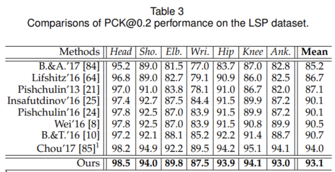
Fig 8. Results on Leeds Sports Poses.
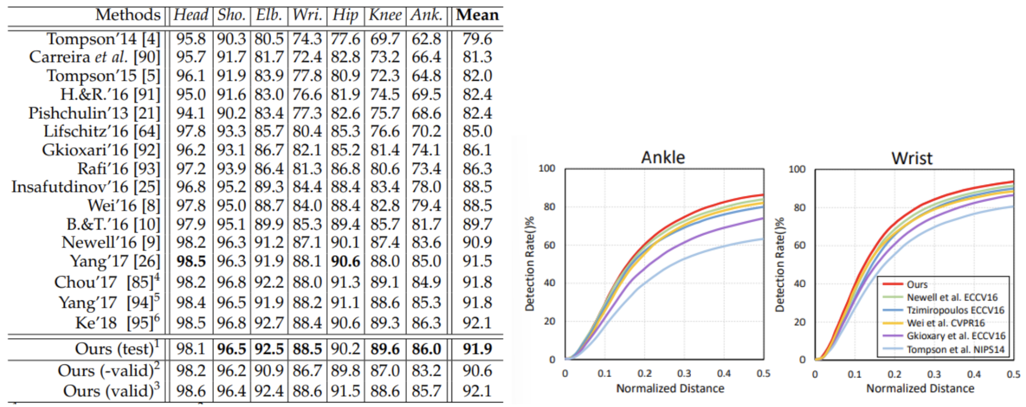
Fig 9. Results on MPII Human Pose
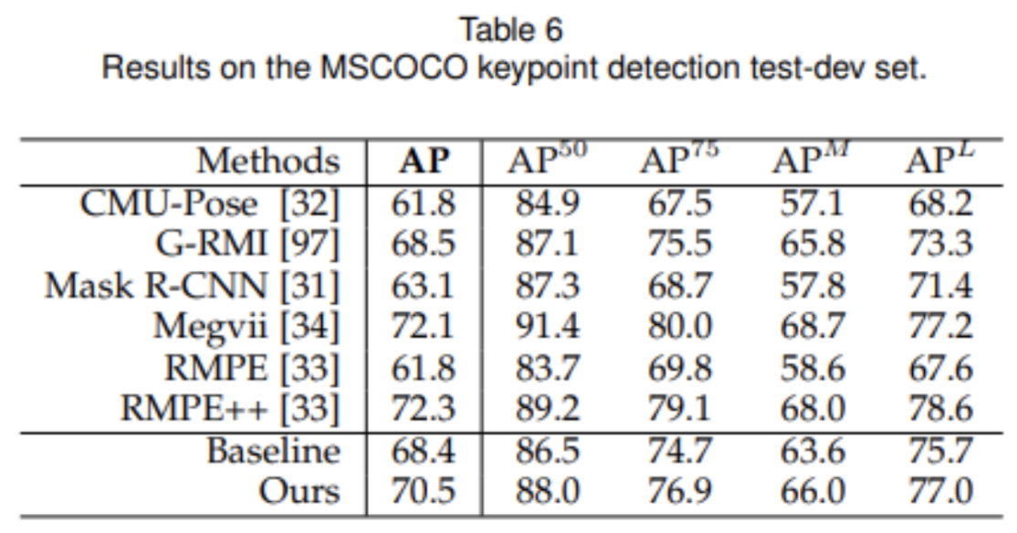
Fig 10. Results on MSCOCO.
Qualitatively, visualizations demonstrated improved handling of occlusions, cropped out body parts, and invisible limbs that raised issues for stacked hourglass. The authors compared a 2-stacked hourglass network to their 2-stacked network and saw better information absorption due to recognizing plausible joint structure.
However, the authors acknowledge their proposal failed in challenging edge cases with twisted limbs at the edge, overlapping people and occluded body parts, and in some cases where the authors speculate a human wouldn’t be able to estimate the pose correctly either.
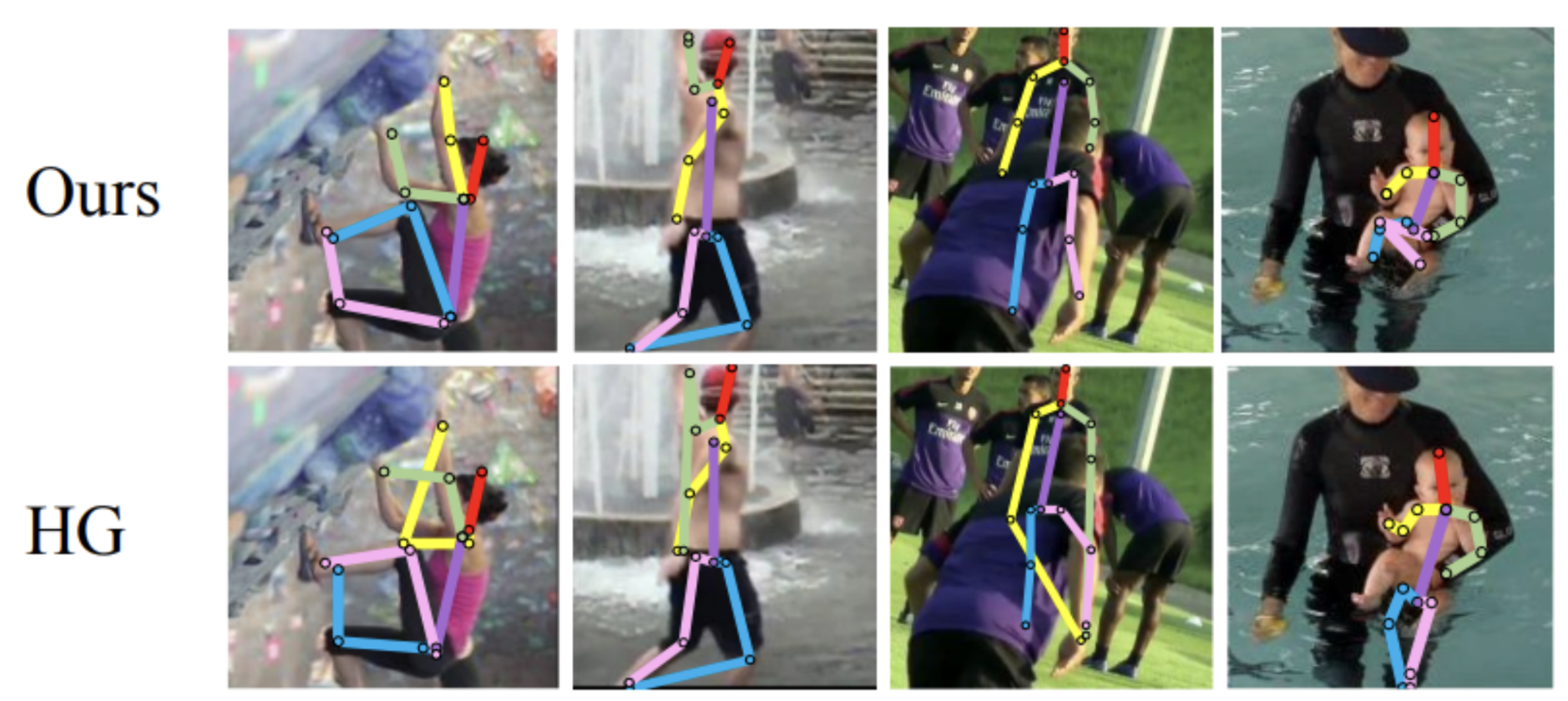
Fig 11. Ours vs HG.
Conclusion
Integration of adversarial learning with fully convolutional networks significantly enhanced pose estimation by leveraging geometric constraints of the human body. The architecture is intuitively designed to mimic the capabilities human vision has in distinguishing plausible postures. To overcome challenges associated with explicitly mathematically modeling, the authors utilize a conditional GAN. Structural priors implicitly encoded within the discriminator coerce the generator to produce biologically plausible poses. This mechanism allows the model to recover from severe occlusions where baseline methods, such as Stacked Hourglass, typically fail. The approach achieved state-of-the-art performance on the MPII and LSP datasets, establishing stacked multi-task and adversarial learning as significant milestones in pose estimation.
YOLO-Pose: Real-Time Multi-Person Pose Estimation
Motivation: why the field swings back toward single-stage efficiency
YOLO-Pose is motivated by a practical bottleneck: the highest-accuracy pipelines in multi-person pose estimation are often multi-stage (detect people, then run a single-person pose model per person), so runtime scales roughly with the number of detected individuals. In contrast, bottom-up approaches run once but rely on non-trivial post-processing (peak finding, refinement, and grouping) that is often non-differentiable and difficult to accelerate. YOLO-Pose targets a middle path: a single forward pass that jointly predicts person boxes and their corresponding 2D skeletons, avoiding per-person reruns and avoiding heavy grouping heuristics.
A key observation is that many challenges in pose estimation mirror those in object detection—scale variation, occlusion, and non-rigid deformation—so the authors argue that advances in object detection should transfer cleanly if pose can be expressed as “detection + structured regression.”
Fig 12. YOLO-Pose highlights "inherent grouping" (keypoints tied to each detected person) vs. bottom-up grouping failures in crowded scenes [4].
Architecture: YOLOv5 as a pose backbone with a keypoint head
YOLO-Pose is built directly on YOLOv5, chosen for its accuracy–compute trade-off on detection. The pipeline keeps the standard YOLOv5 structure—CSP-Darknet53 backbone with PANet feature fusion—and predicts at four scales (feature maps denoted ${P3, P4, P5, P6}$. Each detection head is decoupled into (i) a box head and (ii) a keypoint head.
What changes is the output space per anchor. In YOLOv5 detection, each anchor predicts a vector containing box parameters plus class/objectness terms (for COCO detection, the paper notes 85 elements per anchor in the standard setting). For pose, the task becomes a single class (person) detector with 17 keypoints, and each keypoint has a location and a confidence, totaling 51 keypoint values per anchor. The paper states that the keypoint head predicts 51 elements and the box head predicts 6 elements per anchor.
A clean way to write the per-anchor prediction is:
- Bounding box (6 values): typically representing box geometry + objectness/class terms for the single “person” class (the paper summarizes this as 6 predicted elements).
- Keypoints (51 values): For each of the 17 keypoints, predict (x, y, c), resulting in 17 × 3 = 51 values.
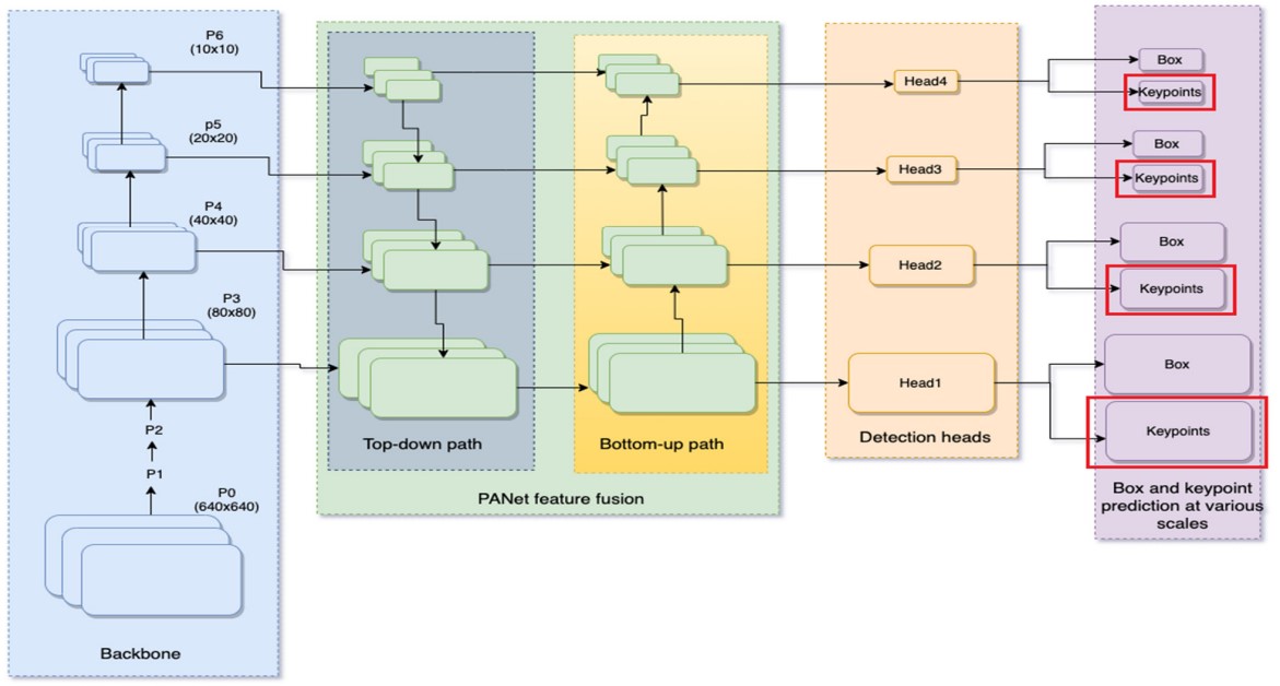
Fig 13. YOLO-Pose extends YOLOv5: CSP-Darknet backbone → PANet fusion → multi-scale heads, each branching into a box head and a keypoint head [4].
Formulation: anchor-based pose as “inherent grouping”
The core modeling decision is: an anchor (or anchor point) matched to a ground-truth person box stores that person’s full pose. This makes the person instance the atomic unit of prediction: keypoints are not predicted “globally” and later assigned; they are predicted conditionally on the anchor/person match.
Concretely, both boxes and keypoints are predicted relative to the anchor center. Box coordinates are transformed with respect to the anchor center, and box dimensions are normalized by anchor size; keypoints are also transformed relative to the anchor center, but (as stated) keypoints are not normalized by anchor width/height. Because the keypoint formulation is not tied to anchor dimensions, the paper argues the approach can transfer to anchor-free detectors as well.
This design directly targets a known failure mode of bottom-up heatmap pipelines in crowds: even if two people’s wrists are spatially close, if they are matched to different anchors, their predictions remain separated (and already grouped).
Keypoint confidence: training signal vs. evaluation signal
Each keypoint includes a confidence c_j. The paper trains this confidence using the dataset’s visibility flags: if a keypoint is visible or occluded, its target confidence is 1; if it is outside the field of view, the target is 0. At inference time, keypoints with predicted confidence (> 0.5) are retained, and the rest are discarded to avoid “dangling” keypoints that would visually deform the skeleton. The paper also notes that this predicted confidence is not used directly in the COCO evaluation, but it is important for filtering out-of-view joints.
Loss design: extending IoU-style supervision from boxes to keypoints
YOLO-Pose mirrors modern detection training by using an IoU-based regression loss for boxes and then introduces the analogous idea for keypoints.
Bounding-box loss (CIoU)
For bounding boxes, the model uses CIoU loss, aligning the regression objective with the scale-invariant overlap-based detection metric family. The paper defines:
\[\mathcal{L}*{\text{box}}(s,i,j,k) = 1 - \mathrm{CIoU}\left(B^{s,i,j,k}*{gt}, B^{s,i,j,k}_{pred}\right)\](where (s) indexes scale and (k) indexes anchors at a grid location).
Keypoint loss (OKS loss as “keypoint IoU”)
The main novelty is to optimize Object Keypoint Similarity (OKS) directly. The authors argue that the commonly used L1 regression loss for keypoints is not equivalent to maximizing OKS: it ignores instance scale and treats all keypoints uniformly, while OKS is scale-normalized and uses keypoint-dependent tolerances (e.g., head keypoints are penalized more for the same pixel error than torso/leg keypoints).
They treat OKS as an IoU-like quantity for keypoints and define the loss as:
\[\mathcal{L}_{\text{kpt}}(s,i,j,k) ;=; 1 - \mathrm{OKS}(s,i,j,k)\]and the paper defines OKS as a sum of exponential penalties applied to normalized squared errors (with visibility gating), meaning keypoints are compared using an exp(·) penalty with scale and keypoint-specific constants.
Two practical claims are emphasized:
- OKS loss is scale-invariant and inherits COCO’s keypoint-wise weighting.
- Unlike vanilla IoU, OKS loss “never plateaus” for non-overlapping cases (the authors compare this behavior to DIoU-style losses).
Keypoint-confidence loss + total loss
The paper adds a confidence loss for keypoints trained from visibility flags (binary classification) and sums losses over scales/anchors/locations. It also reports the balancing weights used in experiments; in their notation, the weights are:
- \[\lambda\_{\text{box}} = 0.5\]
- \[\lambda\_{\text{obj}} = 0.05\]
- \[\lambda\_{\text{kpt}} = 0.1\]
- \[\lambda\_{\text{kpt-conf}} = 0.5\]
as hyperparameters to balance contributions across terms and scales.
Inference and robustness: standard detection post-processing + keypoints beyond the box
A major systems claim is that YOLO-Pose uses standard object-detection post-processing (rather than specialized bottom-up grouping/refinement pipelines). Because keypoints are attached to each detected box/anchor, the output is already instance-separated.
The authors also emphasize a robustness advantage under occlusion: keypoints are not constrained to lie inside the predicted bounding box. If an occluded limb’s keypoint falls outside the visible box extent, YOLO-Pose can still predict it, whereas a strict top-down crop-based pipeline may miss it when the box is imperfect.
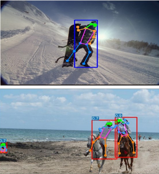
Fig 14. The paper's examples show keypoints predicted outside the detected box under occlusion and imperfect localization [4].
Test-time augmentation: why “no TTA” is a meaningful constraint
The paper argues that many state-of-the-art pose systems rely on test-time augmentation (TTA), especially flip-test and multi-scale testing, to boost accuracy, often at a substantial compute and latency cost. They estimate that flip-test is about 2×, multi-scale testing over scales 0.5, 1, and 2 costs 0.25 + 1 + 4 = 5.25, and combining both results in a 10.5× cost. They also note that the data transforms themselves (flip and resize) may not be hardware-accelerated and can therefore be expensive on embedded devices. All headline results in the paper are reported without TTA.
Experiments: COCO setup and training recipe
The model is evaluated on the COCO Keypoints dataset, which contains over 200k images and about 250k people, each labeled with 17 body keypoints. The dataset is split into train2017 (57k images), val2017 (5k images), and test-dev2017 (20k images). Performance is measured using OKS-based metrics such as AP, AP50, AP75, APL, and AR.
Training follows a setup similar to YOLOv5. Images are augmented using random scaling (0.5 to 1.5), random translation (−10 to 10), horizontal flipping with 50% probability, mosaic augmentation (always applied), and color augmentations. The model is trained using SGD with a cosine learning-rate schedule, a base learning rate of 0.01, and runs for 300 epochs.
At test time, each image is resized so that its longer side matches the target size while keeping the aspect ratio, and then padded to form a square input.
Results: COCO val2017 and test-dev2017 (AP50 + efficiency)
val2017 @ 960 (Table 1): [4]
- YOLOv5s6-pose: AP 63.8, AP50 87.6, 22.8 GMACS
- YOLOv5m6-pose: AP 67.4, AP50 89.1, 66.3 GMACS
- YOLOv5l6-pose: AP 69.4, AP50 90.2, 145.6 GMACS
test-dev2017 (Table 2): [4]
- YOLOv5m6-pose: AP50 89.8
- YOLOv5l6-pose: AP50 90.3
Interpretation: the strong AP50 is attributed to reliable person localization + inherent grouping (keypoints tied to each detected instance), improving looser-threshold precision.
Ablations: what actually matters (loss, resolution, quantization)
(1) OKS loss vs. L1 (Table 3): [4] for YOLOv5-s6 @ 960, OKS gives 63.8 / 87.6, beating L1 58.9 / 84.3 and scale-normalized L1 59.7 / 84.9.
(2) Input resolution (Table 4): [4] accuracy improves with resolution but saturates beyond 960: 640 → 57.5 / 84.3, 960 → 63.8 / 87.6, 1280 → 64.9 / 88.4 (higher GMACS).
(3) Quantization (Table 5): [4] for deployment, they retrain with ReLU (~1–2% drop vs SiLU). 16-bit quantization is essentially lossless (AP 61.8 vs 61.9; AP50 86.7), while 8-bit drops more; mixed precision recovers most performance (60.6 / 85.4) with ~30% layers kept at 16-bit.
Deployability: why ONNX export matters
YOLO-Pose is designed so it can be exported to ONNX from end to end. This is possible because it avoids custom or non-standard post-processing steps that many bottom-up pose methods rely on, such as complex keypoint grouping. As a result, a single exported ONNX model can directly output both bounding boxes and poses, making deployment much simpler, especially on embedded or production systems.
Conclusion
Human pose estimation has evolved significantly from early regression-based approaches like DeepPose to sophisticated architectures that leverage multi-scale reasoning, adversarial learning, and efficient single-stage detection. Stacked Hourglass Networks introduced repeated bottom-up and top-down processing with intermediate supervision, enabling iterative refinement of pose predictions. Adversarial learning approaches further improved robustness by implicitly encoding geometric constraints through discriminator networks, helping models produce anatomically plausible poses even under heavy occlusion. Finally, YOLO-Pose demonstrated that pose estimation can be unified with object detection in a single efficient forward pass, achieving real-time performance while maintaining competitive accuracy. Together, these methods highlight the importance of global context, structural priors, and computational efficiency in human pose estimation.
References
[1] A. Toshev and C. Szegedy, “DeepPose: Human Pose Estimation via Deep Neural Networks,” Proc. IEEE Conf. Computer Vision and Pattern Recognition (CVPR), 2014.
[2] A. Newell, K. Yang, and J. Deng, “Stacked Hourglass Networks for Human Pose Estimation,” Proc. European Conf. Computer Vision (ECCV), 2016.
[3] Y. Chen, C. Wang, B. Han, and J. Liu, “Adversarial Learning of Structure-Aware Fully Convolutional Networks for Landmark Localization,” IEEE Trans. Pattern Analysis and Machine Intelligence (TPAMI), 2019.
[4] D. Maji, S. Nagori, M. Mathew, and D. Poddar, “YOLO-Pose: Enhancing YOLO for Multi-Person Pose Estimation Using Object Keypoint Similarity Loss,” Texas Instruments Inc., 2022.
\[\]