XAI in Facial Recognition
Facial Recognition (FR) systems are being increasingly used in high stake environments, but their decision making processes remain a mystery, raising concerns regarding trust, bias, and robustness. Traditional methods such as occlusion sensitivity or saliency maps (e.g., Grad-CAM), often fail to capture the causal mechanisms driving verification decisions or diagnosis reliance on shortcuts. This report analyzes three modern paradigms that shift Explainable AI (XAI) from passive visualization to active, feature level interrogation. We examined FastDiME [5] which utilizes generative diffusion models to create counterfactuals for detecting shortcut learning, Feature Guided Gradient Backpropagation (FGGB) [3], which mitigates vanishing gradients to produce similarity and dissimilarity maps, and Frequency Domain Explainability [2], which introduces Frequency Heat Plots (FHPs) to diagnose biases in CNNs. By synthesizing these approaches, we examine how modern XAI tools can assess model reliance on noise versus structural identity, with the goal of offering a pathway toward more robust and transparent biometric systems.
- 1. Introduction
- 2. Fast Diffusion-Based Counterfactuals for Shortcut Removal and Generation
- 3. Explainable Face Verification via Feature-Guided Gradient Backpropagation (FGGB)
- 4. Frequency-Domain Based Explainability
- 5. Conclusion
- References
1. Introduction
As Deep Learning models achieve state-of-the-art performance in biometric security, the “black box” nature of Facial Recognition (FR) and Face Verification (FV) systems present a growing liability. Unlike general object classification, FR systems operate in high-risk sociological contexts where errors can lead to wrongful arrests, discriminatory access denial, and security breaches. The challenge is no longer accuracy but trustworthiness to ensure that a model can distinguish identities on robust biometric features rather than spurious “shortcuts” like background textures, lighting artifacts, or demographic biases.
Historically, explainability in computer vision (CV) has relied on saliency methods, such as Grad-CAM [4]. While effective for localizing where a model looks, these methods are fundamentally correlational rather than causal. They often fail to explain why a decision was reached, like whether a match was driven by genuine identity features or coincidental pixel statistics. Furthermore, standard backpropagation methods suffer from noisy or vanishing gradients when applied to deep feature embeddings used in modern FV, rendering conventional heatmaps difficult to interpret for fine-grained verification tasks.
Currently, the landscape of Explainable AI (XAI) is expanding rapidly to address these issues. Researchers are exploring diverse methodologies, ranging from logic-based formal verifications [1] that uses prime implicates to identify minimum sufficient reasons for a classification decision to interactive user interfaces. While these approaches offer promising theoretical guarantees, the need for CV practitioners is often direct feature level diagnostics that can visually and causally verify model behavior.
To address these limitations, this report looks at three methodologies. FastDiME [5] is an approach that leverages diffusion probabilistic models to create counterfactuals. By removing specific attributes and observing a shift, FastDiME offers a causal mechanism for detecting shortcut learning. Feature-Guided Gradient Backpropagation (FGGB) [3], is a different method that shifts focus from final output score to the deep feature level. By normalizing gradients channel-wise, FGGB separates decision-making process into distinct similarity and dissimilarity maps that provide a clearer view of what features argue for or against a match. Frequency Domain Explainability [2] which challenges the spatial bias of human interpretation by analyzing how Convolutional Neural Networks (CNNs) rely on specific frequency bands. This approach reveals that models may rely on high-frequency noise or specific texture patterns offering a powerful tool for quantifying algorithmic bias across different demographics. Together, these methods represent a shift from simple visualization to rigorous feature aware model diagnostics.
2. Fast Diffusion-Based Counterfactuals for Shortcut Removal and Generation
2.1 Introduction
Saliency-based models are among the most popular methods for explainability in computer vision applications. Grad-CAM, for instance, highlights the regions that have the largest effects on model predictions, but doesn’t allow an assessment of how a prediction would change due to the addition or removal of a feature. Beyond saliency by occlusion, current methods cannot help determine whether altering a feature will affect model performance.
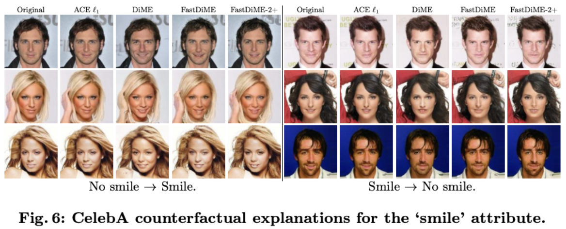
This limitation is especially important in facial recognition tasks, where cues unrelated to facial structure, such as glasses or a mask, could affect model predictions. This methodology proposes a generative approach to explaining model behavior. Instead of relying on visual maps, counterfactual explanations apply a diffusion model to edit the input image to measure the resulting change in prediction. Fast Diffusion-Based Counterfactuals for Shortcut Removal and Generation (FastDiME) generates counterfactuals and uses them to identify “shortcuts,” or features correlated with the label that are not causally relevant.
2.2 Shortcut Learning
Shortcut learning occurs when a vision model uses spurious features that happen to correlate with the label instead of information relevant to the task to identify a class. The paper focuses on medical imaging shortcuts, like pacemakers to correlate with heart disease labels. For facial recognition use cases, shortcuts can include background patterns, accessories, or artifacts from image processing. Objects or patterns unrelated to facial recognition can become correlated with identity.
Shortcuts affect the model’s results when applied to real data where the shortcut is not present. For instance, a facial recognition model could learn to identify a person’s glasses instead of biometric or facial features. Saliency maps can suggest aspects of the face that the model focuses on, but cannot counterfactually confirm whether the model would still recognize the individual without the shortcut. Counterfactual explanations address this by enabling comparisons between model results with and without the shortcut feature.
We can mathematically express shortcut dependence as the sensitivity of the model prediction \(f(x)\)to a shortcut feature\(s\):
\[\Delta_{s}=E_{x}[|f(x)-f(x^{(s\rightarrow\overline{s})})|]\]where \(x^{(s\rightarrow\overline{s})}\)denotes a counterfactual image in which the shortcut feature\(s\) has been removed or altered.
2.3 FastDiME: Guided Diffusion for Counterfactual Faces
The FastDiME framework is built atop diffusion probabilistic models (DDPMs). In a typical DDPM, the model gradually adds Gaussian noise to an image in a forward process, and then learns a reverse process that progressively denoises the image. The forward diffusion process is defined as:
\[q(x_{t}|x_{t-1})=N(x_{t};\sqrt{1-\beta_{t}}x_{t-1},\beta_{t}I)\]Equivalently, the noisy image at time step \(t\) can be written as:
\[x_{t}=\sqrt{\bar{\alpha}_{t}}x_{0}+\sqrt{1-\bar{\alpha}_{t}}\epsilon, \quad \epsilon\sim \mathcal{N}(0,I)\]With:
\[\bar{\alpha}_{t}=\prod_{i=1}^{t}(1-\beta_{i})\]FastDiME changes the reverse process to make a counterfactual image instead of an identical copy. The high-level process is as follows: After noising the input image to an intermediate step, the reverse process is performed with a loss that encourages the removal of a specific feature. The guided mean of reverse diffusion is given by:
\[\mu_{g}(x_{t})=\mu(x_{t})-\Sigma(x_{t})\nabla_{x}\mathcal{L}_{CF}(x_{t})\]The counterfactual is kept as close to the original as possible using a combined loss:
\[\mathcal{L}_{CF}=\lambda_{c}\mathcal{L}_{cls}+\lambda_{1}||x-x_{0}||_{1}+\lambda_{p}\mathcal{L}_{perc}\]FastDiME has a time complexity of \(O(T)\), beating the original DiME with a time complexity of \(O(T^{2})\) by avoiding extraneous inner diffusion calculations that DiME performs during reconstruction.
2.4 Self-Optimized Masking for Localized Image Edits
Using FastDiME to generate images creates the risk that the algorithm alters the facial structure or biometric information entirely as opposed to only the shortcut. Many shortcut features are spatially localized, and therefore, the method introduces a self-optimized mask to restrict changes.
The high-level process is as follows: At each diffusion step, a binary mask is computed by comparing the denoised estimate to the original image:
\[M_{t}=\delta(\overline{x}_{t},x_{0})\]The mask is used to constrain updates so only the masked regions may change:
\[x_{t}^{\prime}=x_{t}\odot M_{t}+x_{t}^{orig}\odot(1-M_{t})\]The mask is updated throughout the diffusion process to encourage localized changes but remove the shortcut feature.
2.5 Quantifying Shortcut Dependence
The paper proposes a quantitative method for classifying the extent to which a classifier is correlated with a shortcut feature. The model is trained with datasets with varied degrees of shortcut-label correlations. Then, counterfactuals are generated based on a balanced test set. The impact is then measured by the change in model predictions between the original and counterfactual images, often using the mean absolute difference (MAD):
\[MAD=E_{x}[|f(x)-f(x^{c})|]\]where \(x^{c}\) represents the removed counterfactual image.
Overall, FastDiME presents a generative and causal approach to explainability for computer vision classifiers, serving as an alternative to saliency-based methods and enabling direct analysis of the features affecting predictions, shortcut dependence, and the robustness of a model.
3. Explainable Face Verification via Feature-Guided Gradient Backpropagation (FGGB)
3.1 Introduction
As Deep Learning models achieve state-of-the-art performance in Face Verification (FV), their lack of transparency remains a critical barrier to deployment. This report examines the landscape of Explainable Face Verification (XFV), specifically addressing the limitations of traditional gradient-based explanation methods. We highlight a novel approach, Feature-Guided Gradient Backpropagation (FGGB), which overcomes the “noisy gradient” problem by shifting the backpropagation focus from the final score to the deep feature level.
This method generates sharper visualizations designed to offer interpretations from the user’s perspective. Specifically, the algorithm aims to explain why the system believes a pair of facial images is matching (“Accept”) or non-matching (“Reject”) by generating precise similarity maps for acceptance decisions and dissimilarity maps for rejection decisions.
3.2 Methodology
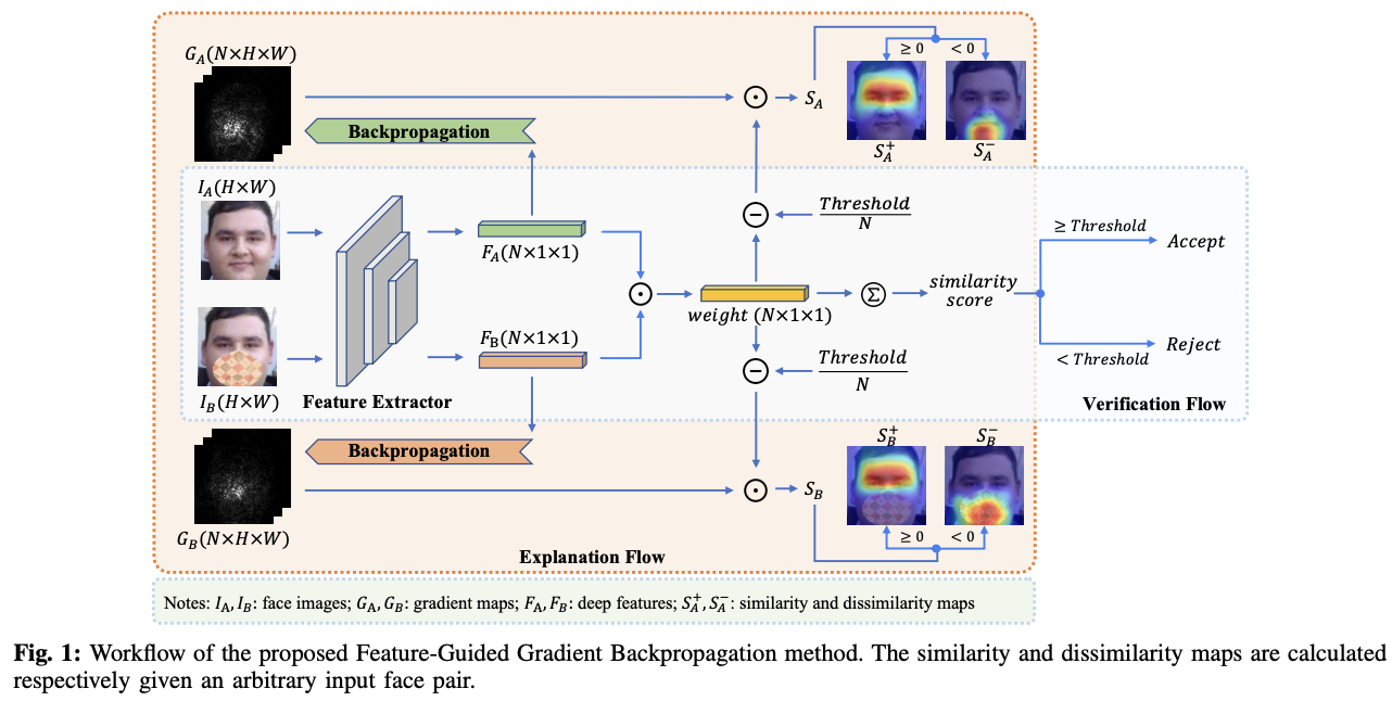
The FGGB method addresses the issue where derivatives of the output score fluctuate sharply or vanish. Instead of backpropagating from the final similarity score, FGGB operates at the deep feature level in a channel-wise manner. The process is divided into two phases:
Gradient Backpropagation & Normalization First, the system extracts the deep face representations (embeddings) for the input images, denoted as \(F_{A}\) and \(F_{B}\) each with dimension \(N\).
-
Gradient Extraction: The system backpropagates gradients from each channel of the feature vector \(F_{A}\). For the \(k\)-th dimension of the feature, the gradient map \(G_{A}^{k}\) is calculated as the derivative with respect to the input image \(I_{A}\):
\[G_{A}^{k}=\frac{\partial F_{A}^{k}}{\partial I_{A}}\] -
Normalization: To mitigate local variations (such as vanishing gradients), each gradient map is normalized using the Frobenius norm to produce \(\overline{G}_{A}^{k}\):
\[\overline{G}_{A}^{k}=\frac{G_{A}^{k}}{\|G_{A}^{k}\|}\]
Saliency Map Generation In the second phase, the system aggregates these \(N\) normalized gradient maps into a final saliency map. The aggregation is weighted by the actual contribution of each feature channel to the verification decision.
-
Weight Calculation: A weight vector is defined as the element-wise cosine similarity between the two feature vectors \(F_{A}\) and \(F_{B}\):
\[weight=\frac{F_{A}\odot F_{B}}{||F_{A}||||F_{B}||}\] -
Weighted Sum: The final saliency map \(S\) is computed by summing the normalized gradient maps. The weights are adjusted by subtracting the decision threshold to distinguish between positive and negative contributions:
\[S_{A}=\sum_{k=1}^{N}\overline{G}_{A}^{k}\cdot(weight_{k}-\frac{threshold}{N})\] -
Map Decomposition: Finally, the map is split into two distinct visualizations:
- Similarity Map (\(S_{A}^{+}\)): Contains positive values, highlighting features that contribute to a match.
- Dissimilarity Map (\(S_{A}^{-}\)): Contains negative values, highlighting features that cause a conflict or rejection.
3.3 Quantitative Evaluation
Validation of the FGGB method was done using the Deletion & Insertion metrics on three datasets (LFW, CPLFW, and CALFW). The “Deletion” metric measures the drop in verification accuracy when salient pixels are removed (lower score is better), while “Insertion” measures accuracy gain when pixels are added (higher is better).
- Performance: FGGB demonstrated superior performance, particularly in generating “Dissimilarity Maps”.
- In the LFW dataset for Similarity Maps, FGGB achieved a Deletion score of 24.18%, significantly outperforming the popular LIME method (35.82%) and performing comparably to perturbation methods like CorrRISE (24.51%) but with much greater efficiency.
- For Dissimilarity Maps (explaining rejections), FGGB achieved a Deletion score of 44.03% on LFW, outperforming the competing gradient-based method xSSAB, which scored 49.72%.
The method’s robustness was validated across different architectures, including ArcFace (99.70% accuracy), AdaFace (99.27%), and MobileFaceNet (98.87%), showing consistent explainability scores across all three.
FGGB bypasses the limitations of score-level backpropagation. By calculating gradients at the feature level and weighting them by their contribution to the cosine similarity, the method successfully generates distinct maps for both matching and non-matching faces. This approach allows for precise, pixel-level explanations of verification decisions without requiring model retraining or expensive iterative perturbations.
4. Frequency-Domain Based Explainability
4.1 Introduction
While methods like FGGB offer precision in the spatial domain, they still operate within a visualization framework that aligns with human intuition. However, a model’s reliance on features is often rooted in the structural information encoded by frequency components, which are invisible in a simple spatial heatmap. To achieve a deeper, mechanistic understanding of feature dependence and model robustness, we shift our focus from pixels and gradients to the frequency domain.
This final method, Frequency Domain Explainability [2], challenges the spatial bias of traditional XAI by analyzing the relative influence of specific frequency bands on verification decisions. By moving beyond where the model looks to what kind of information is driving the decision, this approach offers a powerful new diagnostic tool, especially for quantifying algorithmic bias across different demographics.
4.2 Methodology: Frequency Masking and Influence Scoring
Mathematically, the convolution operation in the spatial domain is equivalent to element-wise multiplication in the frequency domain. Therefore, the learned kernels within a deep network act as filters that selectively emphasize or suppress different spatial frequencies in the input image. These frequencies encode distinct types of image information crucial for recognition, such as fine textures like face wrinkles (high frequency), identifiable features such as eyes and mouth (mid frequency), and overall shapes (low frequency).
The methodology for quantifying frequency influence is perturbation-based and systematic:
- Transformation: The input spatial image is transformed into the frequency domain using the Discrete Fourier Transform (DFT).
- Masking: Specific radial frequency bands are masked (removing information present in those bands). This masked frequency image is then re-transformed back into the spatial domain in a lossless process.
- Scoring: The resulting frequency-masked image, along with the unaltered image, is passed through the FR model to create face embeddings and calculate new cosine similarity scores \(S_{masked}\).
- Influence Score: The importance of the masked frequency band is assessed by taking the difference between the unaltered baseline similarity score \(S_{unaltered}\) and the masked score \(S_{masked}\). This difference is interpreted as the direct influence of that frequency component on the verification decision.
- FHP Generation: The normalized influences are visualized as Frequency Heat Plots (FHPs). These can be Absolute FHPs, which display the magnitude of the performance drop caused by masking a frequency band, or Directed FHPs, showing whether the masking operation worsened the similarity score (positive influence) or improved the score (negative influence).
The detection of negative influence is highly valuable, as it diagnoses scenarios where the model was relying on identity-irrelevant artifacts or noise, which, when removed, stabilizes the decision and increases similarity.
4.3 Key Insights: Diagnosing Structural Bias
The application of this frequency-based approach in extensive experiments on FR models yielded crucial diagnostic insights:
- Differential Feature Reliance: The experiments showed that different frequencies are important to FR models depending on the ethnicity of the input samples. This finding explains algorithmic bias beyond superficial visual factors.
- Quantifying Bias: The differences in frequency importance across demographic groups were observed to increase proportionally with the degree of bias exhibited by the model. This means that frequency importance shifts serve as a measurable metric for diagnosing the structural feature dependencies driving discriminatory behavior.
- Model Vulnerability: The approach was also applied to scenarios like cross-resolution FR and morphing attacks, allowing researchers to understand precisely which frequency bands (e.g., high-frequency texture or low-frequency shape) a model fails to rely on when performance degrades in challenging scenarios.
The research establishes the spatial frequency domain as an essential dimension for explaining the complex decision-making processes of deep learning systems. The introduction of FHPs provides a powerful, quantitative, and diagnostically potent alternative to traditional spatial explanations.
Operationally, the current FHP generation methodology is computationally intensive. For the frequency-domain analysis to become a standard tool in high-throughput operational FR deployments, the field must pursue the development of lightweight, real-time frequency-domain explanation methods that can be integrated directly into the inference pipeline.
5. Conclusion
The analysis reveals a key insight: modern FR models are sensitive to non-semantic cues that escape human notice. While classical models may imply that CNNs “look” at faces much like humans do, recent methods demonstrate that models frequently rely on fragile correlations and spurious shortcuts.
FastDiME’s counterfactual generation proves causality by showing that removing a specific artifact (like glasses or mask) can flip a prediction, while FGGB exposes the precise deep features contributing to false acceptances, and Frequency Heat Plots reveal hidden structural biases across demographics.
Moving forward, the integration of these XAI tools into the standard development pipeline is a must, in order for safe deployment. The shifts from post-hoc visualization to causal and structural analysis allows for detection of time where a model appears correct for the wrong reasons, because they can cause harm in the real world. However, challenges remain regarding computational efficiency. Methods like iterative frequency masking and diffusion-based generation are too expensive for real-time inference. Future research must focus on optimizing these tools to provide real-time feedback ensuring that robustness and fairness are not just retrospective metrics but active components of the recognition process.
References
[1] A. Darwiche, “Logic for explainable AI,” arXiv:2305.05172, May 2023. [Online]. Available: https://arxiv.org/abs/2305.05172
[2] M. Huber, F. Boutros, and N. Damer, “Frequency matters: Explaining biases of face recognition in the frequency domain,” arXiv:2501.16896, Jan. 2025. [Online]. Available: https://arxiv.org/abs/2501.16896
[3] Y. Lu, Z. Xu, and T. Ebrahimi, “Explainable face verification via feature-guided gradient backpropagation,” arXiv:2403.04549, Mar. 2024. [Online]. Available: https://arxiv.org/abs/2403.04549
[4] R. R. Selvaraju et al., “Grad-CAM: Visual explanations from deep networks via gradient-based localization,” International Journal of Computer Vision, vol. 128, no. 2, pp. 336–359, Oct. 2019. [Online]. Available: https://dx.doi.org/10.1007/s11263-019-01228-7
[5] N. Weng et al., “Fast diffusion-based counterfactuals for shortcut removal and generation,” arXiv:2312.14223, Dec. 2023. [Online]. Available: https://arxiv.org/abs/2312.14223