Computer Vision for Medium/Heavy-Duty Vehicle Detection via Satellite Imagery
We fine-tuned a ResNet50-FPN detector on the DOTA aerial dataset and applied it to Google satellite tiles to locate medium/heavy-duty truck parking clusters for EV charging planning.
- 1. Introduction
- 2. Dataset Preparation
- 3. Model Architecture & Training
- 4. Google satellite tile extraction
- 5. Inference & Results
- 6. Conclusion and future work
- 7. References
Computer Vision for Medium/Heavy-Duty Vehicle Detection via Satellite Imagery
Group members:
Rafi Zahedi (805947697)
Aryan Gupta (705943020)
Jace Kasen (205 592 128)
Jacob Young (205 934 037)
1. Introduction
The transportation sector is undergoing a rapid transition toward electrification, with medium- and heavy-duty (MD/HD) vehicles representing one of the most critical and challenging segments to decarbonize. As shown in Fig. 1, these vehicles including Class 3–8 trucks and buses, all above 10,000 lbs GVWR constitute a major share of freight movement in the United States and have a disproportionately large impact on emissions, air quality, and energy demand. California alone hosts approximately 1.8 million trucks, yet as of late 2022 only 1,943 of them were zero-emission, underscoring an enormous electrification gap that must be bridged in the coming decade. Projections show that the state may add 510,000 zero-emission trucks by 2035, scaling to nearly 1.6 million by 2050.
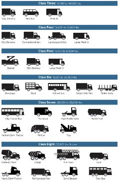
Fig 1. Vehicle classes in the US
A crucial challenge is determining where charging infrastructure should be located to support MD/HD electric vehicle (EV) fleet operations, especially for vehicles that predominantly park outdoors. Satellite imagery offers a scalable and powerful tool to detect the location of MD/HD vehicles before the conversion to the electric models. This helps to detect the high-density locations where are convenient choices to install the charging infrastructure.
This project leverages these properties by training a deep learning model on the DOTA dataset (one of the most frequently used high-resolution aerial imagery datasets with labeled large vehicles), and then applying that model to real-world Google satellite imagery.
Deep learning architectures ResNet-50 with a Feature Pyramid Network (FPN) is well suited for this task because they extract multiscale features and preserve object visibility across wide size variations. Below is the pipeline of this project:
-
Extract and preprocess the DOTA dataset, focusing on MD/HD vehicle classes.
-
Convert annotations to a PyTorch-ready dataset format compatible with modern detectors.
-
Fine-tune a ResNet50-FPN model to learn vehicle features under varying orientations and scales.
-
Apply the trained detector to Google satellite imagery to identify real truck parking clusters across California.
In this project, we built a complete satellite-image detection pipeline to identify MD/HD vehicles for EV-charging planning. We first prepared the DOTA aerial dataset and converted it into a PyTorch-ready COCO format. Using this data, we fine-tuned a Faster R-CNN model with a ResNet-50 + FPN backbone for multi-class vehicle detection. After training the model for 20 epochs, we applied it to a custom Google Maps satellite dataset that we generated by tiling the UCLA campus area—requiring 2,044 image queries. Each tile was analyzed by the model to count MD/HD vehicles, and the results were stored in a CSV file along with geographic coordinates. This allowed me to create a spatial heat map of truck density, which can support future analysis of where heavy-duty EV charging infrastructure may be needed.
2. Dataset Preparation
This section describes the pipeline implemented to convert the DOTA benchmark into a PyTorch-ready classification dataset. The original DOTA dataset consists of very large aerial images, which are annotated with bounding box polygons. Some examples of the object categories include planes, vehicles, and ships. The issue with this dataset is that the images are too large to be fed directly into most deep learning models, and the current annotation format is not applicable for standard PyTorch workflows. The script created provides a solution through tiling large images, converting annotations into COCO format, and creating a PyTorch dataset and dataloader for multi-label classification. code
2.1. Configuration and dependencies
It starts by defining some basic configuration settings that describe where the data lives and where outputs should go. One path points to the overall project directory, another points to the location of the original dataset, which is assumed to contain subfolders for images and their corresponding label files. A separate output directory is specified for all generated results, such as processed images and annotation files, which are stored together in a dedicated folder for the PyTorch‑ready dataset.
A fixed list of DOTA categories is defined, and afterwards, two mappings are created: CAT2ID and ID2CAT. These mappings are used consistently throughout the pipelines, especially in constructing COCO annotations and building multi-label targets.
2.2. Image tilling/ splitting
The first major processing step is tilling the original high-resolution DOTA images into smaller patches. The function split_dota_split handles this for a given split. Three main tiling parameters are defined, which are subsize, gap, and threshold. Gap is the overlap between adjacent tiles,set to 200 pixels; threshold is the minimum fraction of object area that must remain inside a tile for it to be kept. Lastly, the subsize is the tile height/width, set to 1024 pixels. If DOTA_devkit is available, the script constructs a splitbase object using these parameters and invokes its splitdata method. This operation reads from DOTA_ROOT/{split_name} and writes tiles images and corresponding label files into OUTPUT_ROOT/{split)name}_split, preserving the original annotation but clipped to tile boundaries when necessary.
Tiling serves two purposes: it makes the input manageable for neural networks and increases the effective number of training examples, as each large image yields multiple overlapping tiles.
2.3. COCO annotation construction
Once the image tiles have been created, a conversion function turns this tiled dataset into COCO-style JSON annotation files. It assumes a directory structure where one folder contains all tiled images and another folder contains the corresponding text label files. The function goes through every image, records basic information such as unique identifier, file, name, width, and heights, and uses this to build the images section of the COCO dictionary.
For each image, it looks up a matching label file. When a label file is present, it is parsed to extract a set of annotated objects, each described by a quadrilateral polygon and a category name. A helper routine then converts each polygon into an axis-aligned bounding box by finding the minimum and maximum x and y coordinates, and also computes the area of that box.
If an object’s category is part of the predefined class list, the function creates a COCO annotation entry containing a unique annotation id, the image id, the category id, the bounding box, the area, and escrowed flag, and a segmentation field holding the flattened polygon coordinates. All such entries together form the annotations section, while the fixed list of categories becomes the categories section. The combined images, annotation, and categories data structures are then written out as a COCO-style JSON file in an annotations directory.
2.4. PyTorch dataset and DataLoaders
A custom dataset class is used to present the processed tiles in a format compatible with PyTorch. It supports a main way of obtaining labels. It reads a COCO-style annotation file, builds a mapping from each image to all the object categories it contains, and then converts that information into a multi-labeled target vector. This lets a single tile be labeled with multiple object types at once.
3. Model Architecture & Training
3.1. ResNet50
Accurate placement of MD/HD EV charging infrastructure requires reliable data on current truck parking density. We’re using the ResNet50 convolutional network as the backbone for feature extraction, combined with a FPN to handle the scale variation and small object size you get with geospatial images.
Our project needs high precision because infrastructure planning is critical. While ResNet18 was initially suggested as a baseline, we went with ResNet50 to maximize feature robustness, which matters a lot when you’re working with the subtle visual differences in aerial imagery.
ResNet50 has significantly more learnable parameters (23.5 million vs. 11.7 million) and uses the more complex Bottleneck Block design, compared to ResNet18’s simpler Basic Block. This architectural difference gives us two key advantages for our task:
-
Distinguishing a semi-trailer (HD, Class 8) from a large box truck (MD, Class 6) in a low-contrast satellite image means detecting subtle features. The greater depth and parameter count of ResNet50 let it learn a richer, more discriminative representation needed for high-accuracy sub-classification of vehicle types, which is essential for accurate power demand mapping.
-
While ResNet18 offers faster inference, the project’s success depends on the accuracy of the detection and classification. The marginal increase in training time for ResNet50 is worth it for the substantial gain in detection accuracy.
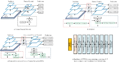
Fig 2. ResNet50 architecture description
3.2. Feature pyramid network (FPN)
Regardless of the backbone depth, the deepest layers of any CNN lose significant spatial resolution (down to 1/32 the size of the input image). For detecting tiny objects like a truck spanning 20×50 pixels, this downsampling kills your performance. The FPN is integrated as the network “neck” to solve this multi-scale detection problem.
FPN builds a feature pyramid by combining two pathways:
- Bottom-up Pathway: The standard feed-forward pass (from the ResNet50 backbone). Resolution decreases, but the feature maps become semantically strong (contextual).
- Top-down Pathway: High-level semantic features from deep layers are upsampled.
- Lateral Connections: The upsampled features are fused with the spatially precise features from the shallower layers via 1×1 convolutions.
This process ensures that every level of the resulting feature pyramid is both semantically rich and spatially precise.
The combination of ResNet50 and FPN is particularly well suited for the project’s core challenge:
- Robust Small Object Detection: The FPN structure ensures that the high-resolution feature maps (like P3 or P4 levels) are semantically informed. This is mandatory for successfully detecting and correctly classifying the tiny vehicle objects in the high-resolution satellite imagery.
- Scale Invariance: FPN allows the detector to effectively handle vehicles of varying sizes and perspectives that appear on the image plane, making the model robust across different parking environments.
- Performance Baseline: The ResNet-FPN pairing is the foundation for industry-leading detectors (like RetinaNet), providing a strong and reliable starting point for training a high-performance, domain-specific model.
4. Google satellite tile extraction
This section describes how we used Google Image API to query from Google, which we use to create a dataset for inferencing in the next section.
The purpose of the get_satellite_image.py utility is to provide a reliable method for data validation. This tool uses the Google Maps Static API to fetch high-resolution satellite imagery for any given geographical coordinate. This allows the team to:
- Validate Detections: When the primary model running on DOTA data yields a low-confidence detection, the corresponding Google image can be fetched to confirm the presence and class (e.g., heavy-duty) of the vehicle.
- Generate Ground Truth: The high-resolution Google images serve as a source for visually verified ground truth data to potentially augment our training set or serve as a high-confidence validation baseline.
The utility is implemented in Python and relies on the requests library to interface with the Google Maps Static API.
Table 1 Google query parameters description
| Parameter | Value | Justification |
|---|---|---|
| maptype | satellite | Specifies the imagery type. |
| zoom | 20 (Max) | Zoom level 20 provides maximum detail, necessary for distinguishing between subtle visual characteristics of medium-duty (Class 3-6) and heavy-duty (Class 7-8) vehicles. |
| size | 640x640 | Standard size for typical computer vision input tiles. |
The script requires a valid Google Maps API Key, which must have the Maps Static API enabled. The key is managed via command line or environment variables for security.
Example Execution: Downloads a satellite image tile centered at 33.7550, -118.2000
python get_satellite_image.py 33.7550 -118.2000 --key “YOUR_API_KEY_HERE”
Output: Saves image to satellite_images/sat_33.7550_-118.2000.png
While the script is functionally complete, its deployment in a batch process faces a severe budgetary constraint based on API usage limits.
- The free tier of the Google Maps Static API allows for 10,000 requests per month. Our project’s ideal validation scope, covering a significant geographic area, is estimated to require 1.5 million requests.
- Beyond the monthly quota, if the script is run in a tight loop to validate thousands of coordinates, the API may enforce burst rate limits, leading to HTTP 429 errors. Any large-scale execution must incorporate exponential backoff or throttling (e.g., using time.sleep) to manage request volume and prevent service denial.
5. Inference & Results
5.1. Model configuration
We fine-tuned a Faster R-CNN detector with a ResNet-50 backbone and FPN using the default COCO pretrained weights. The original classification head was replaced with a new predictor configured for 17 total classes (16 DOTA classes + background). All images were forced to 3-channel RGB using a small wrapper to ensure compatibility with the detector. model
Training parameters were:
-
Optimizer: SGD
-
Learning rate: 0.001
-
Momentum: 0.9
-
Weight decay: 0.0005
-
Batch size: 4
-
Epochs: 20
-
LR schedule: StepLR (step size = 3, gamma = 0.1)
-
Evaluation: Precision/Recall/F1 at IoU ≥ 0.5, score ≥ 0.5
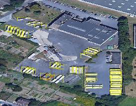
Both train and validation datasets used COCO-format DOTA annotations with only minimal preprocessing (tensor conversion, box cleanup). A model checkpoint was saved after each epoch. Fig. 3 shows the loss reduction per Epoch. Fig. 4 demonstrates the capability of our model in detecting the right object. inference
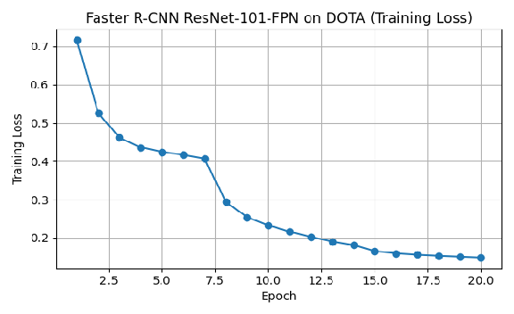
Fig 3. Loss function value per epoch
|  |
|  |
|  |
| :—- | :—- | :—- |
|
| :—- | :—- | :—- |
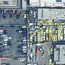
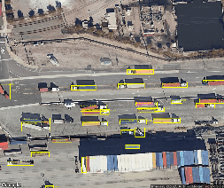
Fig 4. The performance of the fine-tuned model in detecting MD/HD vehicles
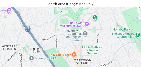
5.2. Google satellite tiling for inference
For inference, we created a Google Maps satellite dataset covering the UCLA campus region from
(34.0789592, −118.4783278) to (34.0603766, −118.419813).
Tiling this bounding box required 2,044 API queries.
Each tile was processed by the trained model, and for every tile we recorded:
-
Tile coordinate (lat/lon)
-
Number of detected MD/HD vehicles
All results were stored in a CSV file, which is used to generate a vehicle density heat map over the UCLA area as shown in Fig. 5.
 |
|---|
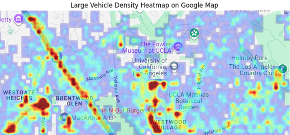 |
Fig 5. High-density location of MD/HD vehicles around UCLA campus
6. Conclusion and future work
This project demonstrated that satellite imagery combined with modern deep learning models can effectively identify MD/HD vehicle activity at a regional scale. By training a ResNet50-FPN detector on the DOTA dataset and applying it to tiled Google imagery of the UCLA area, we generated a spatial map of truck density that can inform early-stage planning for charging infrastructure.
For the future works, we will use the identified locations and the assigned vehicle density to estimate the energy need at each location and plan the local utility grid upgrade to meet that need.
7. References
[1] D. Clar-Garcia, H. Campello-Vicente, M. Fabra-Rodriguez, and E. Velasco-Sanchez, “Research on Battery Electric Vehicles’ DC Fast Charging Noise Emissions: Proposals to Reduce Environmental Noise Caused by Fast Charging Stations,” World Electric Vehicle Journal 2025, Vol. 16, Page 42, vol. 16, no. 1, p. 42, Jan. 2025, doi: 10.3390/WEVJ16010042.
[2] “Alternative Fuels Data Center: Maps and Data - Types of Vehicles by Weight Class.” Accessed: Dec. 12, 2025. [Online]. Available: https://afdc.energy.gov/data/10381
[3] “Public Hearing to Consider the Proposed Advanced Clean Fleets Regulation Staff Report: Initial Statement of Reasons.” Accessed: Dec. 12, 2025. [Online]. Available: https://ww2.arb.ca.gov/sites/default/files/barcu/regact/2022/acf22/isor2.pdf
[4] “DOTA.” Accessed: Dec. 12, 2025. [Online]. Available: https://captain-whu.github.io/DOTA/
[5] P. Y. Chen, J. W. Hsieh, M. Gochoo, C. Y. Wang, and H. Y. M. Liao, “Smaller Object Detection for Real-Time Embedded Traffic Flow Estimation Using Fish-Eye Cameras,” Proceedings - International Conference on Image Processing, ICIP, vol. 2019-September, pp. 2956–2960, Sep. 2019, doi: 10.1109/ICIP.2019.8803719.