Efficient Super-Resolution: Bridging Quality and Computation
Super-resolution has long faced a fundamental tension: the highest-quality models require billions of operations, while edge devices demand sub-100ms inference. This article examines three recent methods—SPAN, EFDN, and DSCLoRa—that challenge this tradeoff through architectural innovation, training-time tricks, and efficient adaptation. We’ll see how rethinking the upsampling operation, leveraging structural reparameterization, and applying low-rank decomposition can each dramatically improve efficiency without sacrificing output quality.
- The Efficiency Problem in Super-Resolution
- Background: The Anatomy of an SR Network
- EFDN: Edge-enhanced Feature Distillation Network for Efficient Super-Resolution (NTIRE 2023 Winner) [1]
- SPAN: Swift Parameter-free Attention Network (NTIRE 2024 Winner) [2]
- DSCLoRa: Efficient Domain Adaptation via Dynamic Sparse Low-Rank Matrices (NTIRE 2025 Winner) [3]
- Conclusion
- References
- References
Image super-resolution is the problem of taking a low-resolution image and turning it into a high-resolution image. Ex. taking a 1080p picture on your cell phone and upscaling it into a beautiful 4K photo. Using deep learning, we can essentially recover detail from the low-resolution input by training a model to learn the relationship between the low- and high- resolution versions of an image.
The Efficiency Problem in Super-Resolution
Leading edge image super-resolution models have gotten very good. Unfortunately, the best models are unsuited to be run on lower-end edge devices due to three main reasons:
- Runtime: models designed to be run on server GPUs will run far slower on edge devices. This makes them unsuitable for real-time or close to real-time applications where the image can’t be shipped off to an inference server
- Parameter Count: edge devices have limited VRAM, RAM, and storage to store the models in, especially considering that they will be running programs other than super-resolution
- FLOPs: edge devices have limited CPU and GPU compute to run models with, especially considering that they will be running other programs
As such, the problem of “efficient image super-resolution” is how to design models to reduce the runtime and parameter count while maintaining some baseline of decent upscaling performance.
The inspiration for this report was the NTIRE Challenge on Efficient Super Resolution (NTIRE ESR), held annually at CVPR. I will analyze three submissions to this challenge, from different years, to compare the differing methods used in recent years to further improve efficient image super resolution models.
Background: The Anatomy of an SR Network
Modern SR networks follow a common template:
Low-Resolution Input → Feature Extraction → Upsampling → High-Resolution Output
Feature extraction uses stacked convolutional blocks to learn hierarchical representations. This is where most computation happens.
Upsampling increases spatial resolution. The dominant method is sub-pixel convolution (pixel shuffle), which:
- Expands channels from \(C\) to \(C \cdot r^2\) (where \(r\) is the scale factor)
- Rearranges these channels into spatial dimensions: \((H, W, C \cdot r^2) \rightarrow (rH, rW, C)\)
This channel expansion is expensive. For \(\times 4\) upsampling with 64 channels, a single \(3 \times 3\) convolution requires: \(64 \times 1024 \times 9 = 589,824 \text{ parameters}\)
In EDSR-baseline (1.37M total parameters), upsampling alone accounts for 31%—nearly a third of the model.
The three papers I analyze optimize different parts of this pipeline.
Background: Measuring Performance
There are many ways to measure the performance of an image super-resolution model. To generate training data, generally the approach is to take a high-resolution image and apply bicubic downsampling to generate the low-resolution version. Then, evaluate the model by applying the model to the low-resolution version and seeing how close the model’s high-resolution generation matches the original high-resolution version.
PSNR (Peak Signal-to-Noise Ratio) compares the “noise” of an image to the original. This noise is calculated using pixel differences between the two images. This is a good measure of pure, mathematical “difference” between two signals, but for images, it should be clear that small differences in pixel values may not matter much. Ex. red 254 vs red 255 is technically a difference, but not very noticeable.
PSNR is measured in decibels (dB), which you will see in the later sections. For the 2025 NTIRE ESR challenge, the submissions were required to have a minimum PSNR of 26.99 on a certain test set.
SSIM (Structural Similarity Index Measure) compares the luminance, contrast, and structure of two images to measure similarity, calculated using the sample means, variances, and covariance of the pixels in both images. It can be thought of as a more higher-level approach as to how similar two images look, vs. how mathematically similar they are.
EFDN: Edge-enhanced Feature Distillation Network for Efficient Super-Resolution (NTIRE 2023 Winner) [1]
The Edge Problem
Efficient SR networks often produce blurry edges. One reason why is that, to the model, edges are not much different than any regular pixels. A one pixel difference in an edge may make it blurry, whereas a one pixel difference in a smooth region may not even be noticeable. Both will be interpreted as similarly bad by the model.
EFDN attempts to solve this from two angles:
- Architecture: Edge-specialized convolution blocks
- Training: Explicit edge supervision via gradient losses
The key innovation is achieving both while minimizing increases to inference cost. At deployment, the edge-specialized convolutions are packed as regular convolutions.
Structural Reparameterization: Training ≠ Inference
EFDN builds on structural reparameterization, similar to RepVGG and DBB. The core idea: train a complex multi-branch architecture, then merge branches into a single convolution for deployment.
During training, EFDN’s EDBB block uses seven parallel branches to enforce explicit edge learning:
Input
  ├── 3×3 Conv (standard features)
  ├── 1×1 Conv (channel mixing)
  ├── 1×1 Conv → 3×3 Conv (expanding-squeezing)
  ├── 1×1 Conv → Sobel-X (learnable horizontal edges)
  ├── 1×1 Conv → Sobel-Y (learnable vertical edges)
  ├── 1×1 Conv → Laplacian (isotropic edges)
  └── Identity (residual)
       ↓
   Output = sum of all branches
Instead of just asymmetric shapes, EFDN leverages Scaled Filter Convolutions. The \(1 \times 1\) convolutions before the fixed edge filters (Sobel/Laplacian) act as learnable scalers, allowing the network to adaptively weight the contribution of specific gradient directions. During inference, all branches (including the fixed filters) are mathematically collapsed into a single \(3 \times 3\) vanilla convolution. Ex.:
\[W_{\text{deploy}} = W_{3 \times 3} + \text{pad}(W_{3 \times 1}) + \text{pad}(W_{1 \times 3}) + W_{\text{identity}}\]where \(\text{pad}()\) zero-pads the asymmetric kernels to \(3 \times 3\), and \(W_{\text{identity}}\) is the identity mapping expressed as convolution weights.The model during training sees seven specialized pathways; the model during inference sees one standard convolution ⟶ Zero overhead.
Edge-Enhanced Gradient Loss
EFDN also introduces explicit edge supervision through loss:
\[\mathcal{L} = \mathcal{L}_{\text{pixel}} + \lambda_x \mathcal{L}_x + \lambda_y \mathcal{L}_y + \lambda_l \mathcal{L}_l\]where:
- \(\mathcal{L}_{\text{pixel}}\): Standard L1 loss on RGB values
- \(\mathcal{L}_x\): L1 loss on horizontal Sobel gradients
- \(\mathcal{L}_y\): L1 loss on vertical Sobel gradients
- \(\mathcal{L}_l\): L1 loss on Laplacian (edge localization)
The Sobel operators detect gradients: \(S_x = \begin{bmatrix} -1 & 0 & 1 \\ -2 & 0 & 2 \\ -1 & 0 & 1 \end{bmatrix}, \quad S_y = \begin{bmatrix} -1 & -2 & -1 \\ 0 & 0 & 0 \\ 1 & 2 & 1 \end{bmatrix}\)
The Laplacian detects edges regardless of orientation: \(L = \begin{bmatrix} 0 & 1 & 0 \\ 1 & -4 & 1 \\ 0 & 1 & 0 \end{bmatrix}\)
The authors use these filters to calculate gradient maps. These maps are then unfolded into patches, the patches used to calculate gradient variances, the variances used to calculate gradient variance loss for each of the three filters.
\[\begin{align} \mathcal{L}_{x} &= \mathbb{E}_{I^{SR}} \| v_{x}^{HR} - v_{x}^{SR} \|_{2} \\ \mathcal{L}_{y} &= \mathbb{E}_{I^{SR}} \| v_{y}^{HR} - v_{y}^{SR} \|_{2} \\ \mathcal{L}_{l} &= \mathbb{E}_{I^{SR}} \| v_{l}^{HR} - v_{l}^{SR} \|_{2} \end{align}\]By minimizing gradient errors directly, the network learns to preserve high-frequency details that pixel-only losses would smooth over.
Hyperparameter Analysis
The paper experiments with different \(\lambda\) values:
| \(\lambda_x = \lambda_y\) | \(\lambda_l\) | Set5 PSNR | Visual Quality |
|---|---|---|---|
| 0.1 | 0.05 | 32.15 dB | Slight blur |
| 0.2 | 0.1 | 32.19 dB | Sharp edges |
| 0.3 | 0.15 | 32.17 dB | Oversharpened |
| 0.5 | 0.2 | 32.03 dB | Ringing artifacts |
The authors decided on a sweet spot of \(\lambda_x = \lambda_y = 0.2\), \(\lambda_l = 0.1\). Too high causes ringing; too low reverts to pixel-loss behavior.
Quantitative Results
Comparison on \(\times 4\) SR benchmarks:
| Method | Params | Multi-Adds | Set5 | Urban100 | Inference (RTX 3090) |
|---|---|---|---|---|---|
| CARN | 1,592K | 90.9G | 32.13 dB | 26.07 dB | - |
| IMDN | 715K | 41.0G | 32.13 dB | 26.04 dB | 92 ms |
| PAN | 272K | 28.2G | 32.13 dB | 26.11 dB | - |
| EFDN | 276K | 14.7G | 32.08 dB | 26.00 dB | 19 ms |
EFDN achieves the best efficiency: ~2.5x fewer Multi-Adds than IMDN and significantly faster inference (19ms vs 92ms), while maintaining comparable quality.
Ablation Study: (Scale \(\times 2\))
As is standard, the authors performed an ablation study to test the improvements from each new addition independently, then all togehter.
| Configuration | Set5 PSNR | Inference Cost |
|---|---|---|
| Baseline (\(L_1\)) | 37.09 dB | Baseline |
| + Edge Loss (\(L_{EG}\)) | 37.14 dB | +0 ms |
| + Edge Blocks (EDBB) | 37.19 dB | +0 ms |
| + Both (EFDN strategy) | 37.27 dB | +0 ms |
The edge blocks and edge loss are complementary:
- EDBB: Adds structural extraction capacity (Sobel/Laplacian branches) that collapses to a single conv at inference.
- \(L_{EG}\): Calibrates the training of these branches to focus on gradient variance.
Together they achieve consistent improvement (+0.18 dB) at zero additional inference cost.
SPAN: Swift Parameter-free Attention Network (NTIRE 2024 Winner) [2]
Attention mechanisms have become increasingly important to achieve high-quality super resolution. Architectures like RCAN or SwinIR leverage channel or spatial attention to focus processing power on high-frequency details (textures, edges) rather than smooth backgrounds.
However, attention mechanisms are computationally expensive. SPAN attempts to replicate the benefits of attention without dramatically increasing the complexity and parameter count of the model.
SPAN’s fundamental hypothesis is that the network doesn’t need a separate branch to tell it which features are important. In Convolutional Neural Networks (CNNs), feature magnitude is already a proxy for importance. In SR tasks, “information-rich” regions like edges and complex textures typically trigger high-magnitude activations in convolutional filters (similar to how a Sobel filter reacts strongly to an edge). SPAN leverages this by deriving the attention map directly from the feature map itself, eliminating the need for extra learnable weights.
SPAB: the Swift Parameter-free Attention Block
The backbone of SPAN consists of cascaded Swift Parameter-free Attention Blocks (SPABs). Unlike traditional blocks that use separate pathways for attention, SPAB integrates it directly into the feature extraction flow.
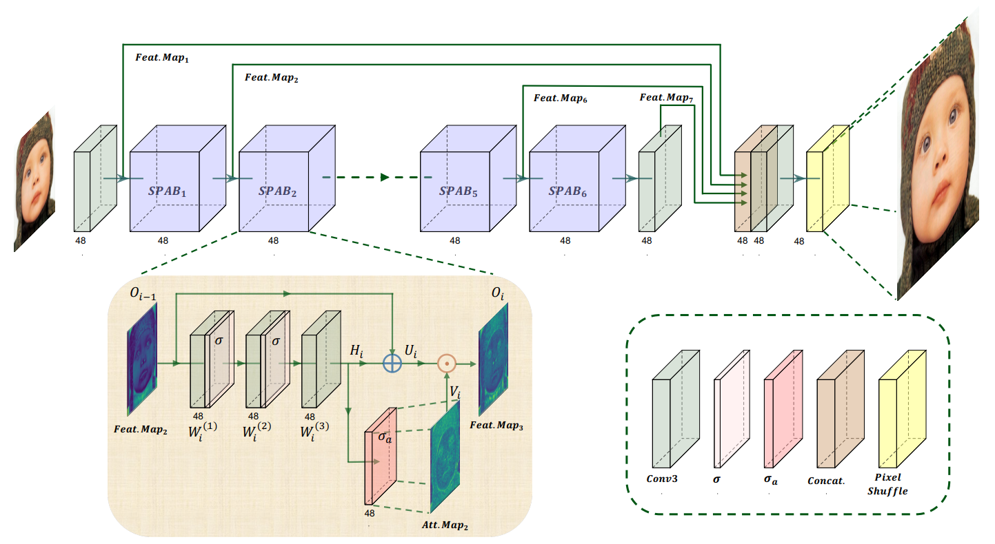
Fig 1. SPAN: architecture design.
Essentially, SPAB applies an activation function on the feature map to generate an attention map. This attention map is then element-wise multiplied with the (feature map + residual connection) to get the output of the SPAB block.
High magnitude activations in a CNN feature map generally correspond to important features like edges, keypoints, etc. The authors wanted an activation function that kept these high magnitude activations while suppressing near-zero activations. The sign of the activation also should not matter, since key features generate high magnitude activations regardless of sign (ex. a Sobel filter detects an edge no matter if the edge is oriented one way or the other). Thus, the activation function should be odd-symmetric.
After experimentation, the authors settled on a shifted sigmoid to generate the attention map \(V_i\):
\(\sigma_a(x) = \text{Sigmoid}(x) - 0.5\) By shifting the Sigmoid, the function becomes odd-symmetric about the origin. This ensures that features with high absolute magnitudes (whether positive or negative) generate significant responses in the attention map, while near-zero values (smooth background regions) are suppressed.
Mathematical Intuition: Self-Supervised Gradient Boosting
The paper provides a theoretical analysis of why this works. When using this attention mechanism, the gradient used to update the weights during training is scaled by the attention map itself.
Mathematically, the gradient term effectively becomes proportional to the activation magnitude. This means the network naturally receives stronger supervision signals in information-rich regions (edges/textures) and weaker signals in smooth regions. It acts as a form of self-supervised hard-example mining, forcing the network to “try harder” on difficult textures without explicit guidance.
Architectural Nuances
The “Forgetfulness” Problem & Residual Connections One danger of attention mechanisms is that they act as filters. By aggressively modulating features, deep networks can inadvertently suppress low-level information needed for reconstruction. SPAN solves this by adding a residual connection within the attention block.
- Mechanism: The input to the block (\(O_{i-1}\)) is added to the extracted features (\(H_i\)) before the attention modulation is applied.
- Result: This ensures that even if the attention map suppresses the current layer’s output, the original information flows through, preventing the “vanishing feature” problem common in deep attention networks.
- Testing: From the authors’ testing, the residual connections substantially increased the ability of the attention mechanism to retain information
Structural Re-parameterization To further boost speed, SPAN employs structural re-parameterization (similar to RepVGG).
Experimental Results:
SPAN won 1st place in both the Overall Performance and Runtime tracks of the NTIRE 2024 Efficient Super-Resolution Challenge.
Performance vs. Latency Trade-off (\(\times 4\) Upscaling):
| Method | Parameters | Inference Speed (RTX 3090) | PSNR (Urban100) |
|---|---|---|---|
| IMDN | 715K | 20.56 ms | 26.04 dB |
| RLFN | 543K | 16.41 ms | 26.17 dB |
| SPAN | 498K | 13.67 ms | 26.18 dB |
Key Takeaways:
- Fastest in Class: SPAN runs ~15% faster than RLFN and ~33% faster than IMDN while using fewer parameters.
- Visual Quality: Qualitative comparisons show that SPAN reconstructs sharper lattice structures (e.g., building windows in Urban100) where other lightweight models suffer from aliasing or blurring.
- Real-World Viability: By removing the “latency tax” of attention, SPAN proves that high-performance SR is feasible on constrained hardware without sacrificing the benefits of content-aware processing.
DSCLoRa: Efficient Domain Adaptation via Dynamic Sparse Low-Rank Matrices (NTIRE 2025 Winner) [3]
Winner of the NTIRE 2025 Efficient Super-Resolution Challenge (Overall Performance Track), DSCLoRA introduces a framework to fine-tune lightweight models (specifically SPAN) using Low-Rank Adaptation supervised by a massive teacher network. Through these methods, we are able to squeeze more performance out of existing architectures.
Innovation 1: ConvLoRA & SConvLB
While LoRA is famous in the LLM world for fine-tuning transformers, DSCLoRA adapts it for Convolutional Neural Networks (CNNs) via the SConvLB (Super-resolution Convolutional LoRA Block).
The Mechanism: Standard LoRA approximates weight updates using low-rank matrices. DSCLoRA applies this to convolution kernels. For a frozen pre-trained convolution weight \(W_{PT}\), the update is modeled as:
\[W_{\text{updated}} = W_{PT} + X \times Y\]where \(Y\) (initialized to zero) and \(X\) (random Gaussian) are low-rank matrices (\(r \ll \text{channel dimension}\)).
Zero-Overhead Inference: Because convolution is a linear operation, the learned low-rank weights (\(X \times Y\)) can be mathematically merged into the original frozen weights:
\[W_{\text{final}} = W_{PT} + (X \times Y)\]During inference, the auxiliary LoRA branches are removed. The model architecture remains identical to the original lightweight baseline, meaning zero additional FLOPs and zero extra inference latency, despite the performance boost.
Innovation 2: Spatial Affinity Distillation
Simply adding LoRA layers isn’t enough to achieve state-of-the-art results. The authors found that pixel-wise loss functions (L1/L2) fail to capture the high-frequency structural details essential for super-resolution.
To solve this, DSCLoRA employs Spatial Affinity Knowledge Distillation (SAKD).
How it works: Instead of forcing the student (DSCLoRA) to mimic the teacher’s (Large SPAN) raw feature maps, it forces the student to mimic the teacher’s spatial relationships.
- Feature maps \(F \in \mathbb{R}^{C \times H \times W}\) are flattened.
- An affinity matrix \(A \in \mathbb{R}^{HW \times HW}\) is computed, representing the pairwise similarity between every spatial location in the image.
- The distillation loss minimizes the distance between the Student’s and Teacher’s affinity matrices:
This transfers the “structural knowledge” (texture patterns, edge continuity) from the heavy teacher to the lightweight student, guiding the optimization of the LoRA parameters.
Architecture: The “SConvLB” Upgrade
The framework is built upon the SPAN (Swift Parameter-free Attention Network) architecture. DSCLoRA modifies it by:
- Replacing Blocks: Standard SPAB blocks are replaced with SConvLB blocks containing the parallel LoRA branches.
- Applying ConvLoRA to the main feature extraction convolutions and the critical upsampling (PixelShuffle) layers.
- Better Training: The backbone weights are frozen; only the small LoRA parameters are updated.
Experimental Results
The method was evaluated on standard SR benchmarks (\(\times 4\) scale), comparing the original lightweight SPAN against the DSCLoRA-enhanced version.
Quantitative Performance (Manga109):
| Model | Params (Inference) | FLOPs | PSNR | SSIM |
|---|---|---|---|---|
| SPAN-Tiny (Baseline) | 131K | 8.54G | 29.56 dB | 0.8967 |
| DSCLoRA (Ours) | 131K | 8.54G | 29.60 dB | 0.8971 |
Some takeaways:
- Both models have the exact same parameter count and FLOPs during inference.
- DSCLoRA achieves consistently higher PSNR/SSIM across all benchmarks (Set5, Set14, Urban100, Manga109).
- Qualitative comparisons show DSCLoRA recovers finer details (e.g., building lattices, animal fur) where the baseline and other lightweight models (like RFDN or RLFN) produce aliasing or blur.
Why does this matter?
Nevertheless, DSCLoRA (using SPAN Tiny) won the NTIRE 2025 ESR Challenge, beating out SPANF, a further optimized version of SPAN from the original authors.
DSCLoRA shifts the focus from architecture design to training dynamics. It proves that existing efficient architectures are often under-optimized. By using a temporary, high-capacity training setup (Teacher + LoRA) that collapses into a simple deployment model, we can achieve superior results on resource-constrained devices without any hardware penalties.
Conclusion
Overall, we’ve seen impressive growth in efficient super resolution models. PSNR/SSIM is just as good or better while models have achieved ~5x reductions in parameter size and runtime. There is a lot of optimizations to be gained, whether through better architectures (focusing on edges or attention maps), more nuanced loss functions, or additional work put into finetuning and further training models.
References
References
[1] Y. Wang, “Edge-Enhanced Feature Distillation Network for Efficient Super-Resolution,” in Proceedings of the IEEE/CVF Conference on Computer Vision and Pattern Recognition (CVPR) Workshops, 2022, pp. 777-785.
[2] C. Wan, H. Yu, Z. Li, Y. Chen, Y. Zou, Y. Liu, X. Yin, and K. Zuo, “Swift Parameter-free Attention Network for Efficient Super-Resolution,” in Proceedings of the IEEE/CVF Conference on Computer Vision and Pattern Recognition (CVPR), 2024, pp. 6246–6256.
[3] X. Chai, Y. Zhang, Y. Zhang, Z. Cheng, Y. Qin, Y. Yang, and L. Song, “Distillation-Supervised Convolutional Low-Rank Adaptation for Efficient Image Super-Resolution,” arXiv preprint arXiv:2504.11271, 2025. [Online]. Available: https://arxiv.org/abs/2504.11271