Depth From Stereo Visions
Our project explores the use of Deep Learning for inferring the depth data based on two side-by-side camera images. This is done by determining which pixels on each image corresponding to the same object (a process known as stereo matching), and then calculating the distance between corresponding pixels, from which the depth can be calculated (with information about the placement of the cameras). While there exist classical vision based solutions to stereo matching, deep learning can produce better results.
Background
Stereo matching is the process of aligning two images taken by distinct cameras of the same object. In the very simple case, with perfect images, and one object at constant depth, one can compute the disparity (pixel alignment offset) required to align both the left and right camera images. This information can be used, along with the distance between the two cameras, to compute a distance estimation for this object. In the real world case, this problem becomes much more complicated. Many objects reside in the scene with different textures, shadows, etc, and performing an alignment between all these points is difficult, making it more challenging to estimate distance than in the simple case.
There are two different forms of stereo matching: active and passive. In the active case, one simplifies the problems of alignment by projecting light (often via a laser dot matrix) and using other adaptive mechanisms to make it easier to align the two camera images. This hardware is much more expensive however and thus not as likely to see widespread use. Passive stereo imaging just involves two statically placed cameras and thus is a much harder problem that we will explore for our final project.
A natural question that also might be asked, is why not use a single camera for depth estimation? There are some models that explore this, but it is much more difficult to get accurate depth measurements, and there is a large gap between depth accuracies (as shown in [4]).
Model Choice
We evaluated multiple different papers when deciding on what we wanted to choose for our final project. As we were particularly interested in stereo depth matching for robotics applications, we favored algorithms that could run in close to real time, so we’d be able to observe the depth estimations of objects as we walked by them. We considered both HITNet (a recent network, although admittedly a somewhat complex one) authored this year by Google, and StereoNet (a model which uses a 2 pass Siamese Network). The HITNet model seemed like a good choice due to its adaptation of many techniques used in conventional active stereo matching to the passive stereo matching field, as well as its omission of a cost volume (a common source of expense in stereo matching models due to the need to use 3D convolutions). StereoNet also seemed like a reasonable choice as it was a much simpler and understandable model that instead solved the problem of expensive cost volume computation by heavily downsampling the input image and using refinement on this output with the original input images. As these models take fundamentally different approaches, we figured understanding them would give us a good overview of the stereo depth matching problem.
HITNet
HITNet is a recent model that works to use some of the recent techniques from active stereo depth applied to the passive stereo problem. It is optimized for speed, using a combination of a fast multi-resolution initial step, and 2d disparity propagation, instead of much more costly 3D convolutions. Although it performs slightly worse than the 3D convolutional models, it takes only milliseconds to process an image pair, compared to seconds from those models.
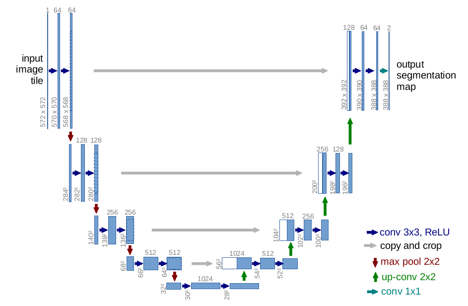
This is the UNet feature extractor implementation used in the HITNet model. It has 4 stages of downsampling and upsampling. It also uses LeakyReLU activation with 0.2 slope for improved training.
class UpsampleBlock(nn.Module):
    def __init__(self, c0, c1):
        super().__init__()
        self.up_conv = nn.Sequential(
            nn.ConvTranspose2d(c0, c1, 2, 2),
            nn.LeakyReLU(0.2),
        )
        self.merge_conv = nn.Sequential(
            nn.Conv2d(c1 * 2, c1, 1),
            nn.LeakyReLU(0.2),
            nn.Conv2d(c1, c1, 3, 1, 1),
            nn.LeakyReLU(0.2),
            nn.Conv2d(c1, c1, 3, 1, 1),
            nn.LeakyReLU(0.2),
        )

    def forward(self, input, sc):
        x = self.up_conv(input)
        x = torch.cat((x, sc), dim=1)
        x = self.merge_conv(x)
        return x
Initialization
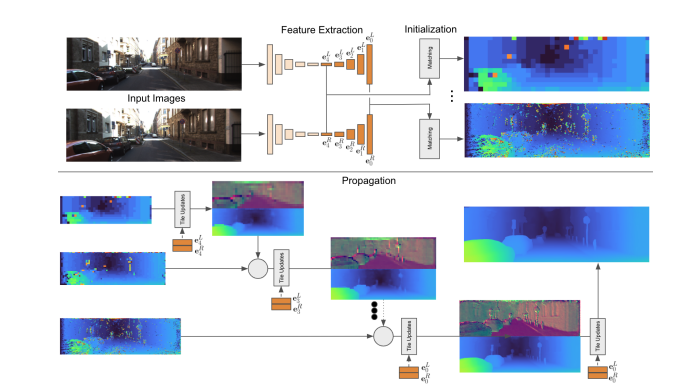
The key idea of the initialization step of HITNet is the use of an encoder decoder network, with the model using the results of all the different resolution layers output by the encoder. The initialization phase builds on top of U-Net (such a decoder-encoder network) which is shown in Figure 1. After generating different resolution features for both \(I_R\) and \(I_L\) (the left and right images) we obtain two multiscale representations denoted \(\epsilon^R\) and \(\epsilon^L\). Taking \(\epsilon^R\) and \(\epsilon^L\) we then attempt to align tiles of these images. The idea here is for each resolution, we want to tile that image and map tiles in \(\epsilon^L\) to \(\epsilon^R\). We denote the feature map for a specific resolution l as \(e_l\).
class FeatureExtractor(nn.Module):
    def __init__(self, C):
        super().__init__()
        self.down_0 = nn.Sequential(
            nn.Conv2d(3, C[0], 3, 1, 1),
            nn.LeakyReLU(0.2),
        )
        self.down_1 = nn.Sequential(
            SameConv2d(C[0], C[1], 4, 2),
            nn.LeakyReLU(0.2),
            nn.Conv2d(C[1], C[1], 3, 1, 1),
            nn.LeakyReLU(0.2),
        )
        self.down_2 = nn.Sequential(
            SameConv2d(C[1], C[2], 4, 2),
            nn.LeakyReLU(0.2),
            nn.Conv2d(C[2], C[2], 3, 1, 1),
            nn.LeakyReLU(0.2),
        )
        self.down_3 = nn.Sequential(
            SameConv2d(C[2], C[3], 4, 2),
            nn.LeakyReLU(0.2),
            nn.Conv2d(C[3], C[3], 3, 1, 1),
            nn.LeakyReLU(0.2),
        )
        self.down_4 = nn.Sequential(
            SameConv2d(C[3], C[4], 4, 2),
            nn.LeakyReLU(0.2),
            nn.Conv2d(C[4], C[4], 3, 1, 1),
            nn.LeakyReLU(0.2),
            nn.Conv2d(C[4], C[4], 3, 1, 1),
            nn.LeakyReLU(0.2),
            nn.Conv2d(C[4], C[4], 3, 1, 1),
            nn.LeakyReLU(0.2),
        )
        self.up_3 = UpsampleBlock(C[4], C[3])
        self.up_2 = UpsampleBlock(C[3], C[2])
        self.up_1 = UpsampleBlock(C[2], C[1])
        self.up_0 = UpsampleBlock(C[1], C[0])

    def forward(self, input):
        x0 = self.down_0(input)
        x1 = self.down_1(x0)
        x2 = self.down_2(x1)
        x3 = self.down_3(x2)
        o0 = self.down_4(x3)
        o1 = self.up_3(o0, x3)
        o2 = self.up_2(o1, x2)
        o3 = self.up_1(o2, x1)
        o4 = self.up_0(o3, x0)
        return o4, o3, o2, o1, o0
To get the tile features we run a 4x4 convolution on both \(\epsilon^L\) and \(\epsilon^R\), but there’s a subtle point here: We want to cover our features with overlapping tiles, but we also want to minimize the number of disparity values we have to try. In order to solve this problem the authors introduce the following asymmetry, when applying the convolution on the selected tile regions from the feature map. For \(\epsilon^L\) overlap the tiles in x direction and use a 4x4 stride on the convolution. For \(\epsilon^R\) do not overlap the tiles, but instead use a 4x1 stride in the convolution so the tiles overlap in the convolution computation. This allows us to formulate our matching cost c for a specific location (x,y) with resolution l and disparity d as: \(c(l,x,y, d) = \lvert \lvert e_{l,x,y} - e_{l, 4x -d, y} \rvert \rvert_1\) We then compute the disparities for each (x,y) location and resolution l, where D is the max disparity, noting that our convolution trick allows us to try far fewer values for the disparity with the following:
\[d_{l,x,y}^{init} = argmin_{d \in [0,D]}c(l,x,y,d)\]This search is exhaustive over all potential disparity values.
The authors also add an additional parameter to the model which they denote the tile feature descriptor \(p_{l,x,y}^{init}\) for each point (x,y) and resolution l. This is a value which is the output of a perceptron and leaky ReLU fed the costs of the best matching disparity d, and the embedding for that specific feature at that point. The idea of this feature is to pass along the confidence of the match to the network layers.
Propagation
Warping
The second step of the model, propagation, uses input from all the different resolutions of the features. First we perform a warping between the individual tiles that are associated with each feature resolution using the computed disparity values from before. We warp the tiles in the right tile features \(e^R\) to the left tile features \(e^L\) (converting them into their original size on the feature map) using linear interpolation along the scan lines. To pass this information on to the next iteration of the algorithm a cost vector is also computed which takes the magnitude of the distance between all of the feature values in this 4x4 tile.
@functools.lru_cache()
@torch.no_grad()
def make_warp_coef(scale, device):
    center = (scale - 1) / 2
    index = torch.arange(scale, device=device) - center
    coef_y, coef_x = torch.meshgrid(index, index)
    coef_x = coef_x.reshape(1, -1, 1, 1)
    coef_y = coef_y.reshape(1, -1, 1, 1)
    return coef_x, coef_y


def disp_up(d, dx, dy, scale, tile_expand):
    n, _, h, w = d.size()
    coef_x, coef_y = make_warp_coef(scale, d.device)

    if tile_expand:
        d = d + coef_x * dx + coef_y * dy
    else:
        d = d * scale + coef_x * dx * 4 + coef_y * dy * 4

    d = d.reshape(n, 1, scale, scale, h, w)
    d = d.permute(0, 1, 4, 2, 5, 3)
    d = d.reshape(n, 1, h * scale, w * scale)
    return d
Update
A CNN model \(U\) then takes n tile hypotheses as input and predicts a change for the tile plus a confidence value \(w\). This convolutional layer is useful as it allows the use of neighboring information from other tiles, along with the multidimensional inputs to be used in updating the tile hypothesis. The tile hypothesis is augmented with the matching costs \(\phi\) computed during the warping step, with the warp costs stored for the current estimate and offset +-1 to give a local cost volume. This allows the disparity value to be iteratively updated at different scales without the need for an explicit cost volume. In the paper the augmented tile map is denoted as follows:
\[a_{l,x,y} = [h_{l,x,y}, \phi(e_l, d - 1), \phi(e_l, d), \phi(e_l, d +1)]\]Our model then outputs deltas for each of the n tile hypothesis maps and new confidence values as shown here:
\[(\Delta h_l^1, w^1, \cdots, \Delta h_l^n, w^n) = U_l(a_l^1, \cdots, a_l^n; \theta_{U_l})\]The CNN model \(U\) is made of ResNet blocks followed by dilated convolutions. The update is performed starting at lowest resolution feature, moving up, so at the second resolution feature there are now two inputs, and then three, and so on and so forth. This action can be seen in Figure 2. Tiles are upsampled as they move up layers to ensure they all stay the appropriate dimension. At each location the hypothesis with the largest confidence is selected until the starting resolution is reached. The model is then run one additional time on the optimal tiles for further refinement and the final output is the disparity map result.
Loss
The network uses multiple different losses: an initialization loss, propagation loss, slant loss, and confidence loss. These values are all weighted equally and used to optimize the model.
Initialization Loss
The ground truth disparity values are given with subpixel precision, but the model only generates integer disparities. To account for this the authors used linear interpolation to compute the matching costs for subpixel disparities via the given equation (subscripts omitted for brevity).
\[\psi(d) = (d - \lfloor d \rfloor)\rho(\lfloor d \rfloor + 1) +(\lfloor d \rfloor + 1 - d) \rho(\lfloor d \rfloor)\]In order to compute the disparity cost at multiple resolutions the ground truth disparity maps are maxpooled to downsample them to the appropriate resolution. The goal is for the loss $\psi$ to be the smallest for the ground truth disparity and greater everywhere else. The authors achieved this goal by using an $l_1$ contrastive loss as defined below.
\[L^{init}(d^{gt}, d^{nm}) = \psi(d^{gt}) + \text{max}((\beta - \psi(d^{nm}), 0)\]Where $\beta > 0$ is a margin (the authors’ use $\beta = 1$ in the paper), $d^{gt}$ is the ground truth disparity and:
\[d^{nm} = \text{argmin}_{d \in [0, D] \setminus \{d:d \in [d^{gt} - 1.5, d^{gt} 1.5]\}}\rho(d)\]where \(d^{nm}\) is the disparity of the lowest cost match for a location. By defining the cost this way the lowest cost match approaches the margin and the ground truth cost approaches 0.
Propagation Loss
To apply loss on the tiles the authors expand the tiles to the full resolution disparities. They also upsample the slant to full-resolution using nearest neighbors. The paper uses a general robust loss function (also used in StereoNet) and defined as $\rho$ and apply a truncation to this loss with a threshold $A$.
\[L^{prop}(d, dx, dy) = \rho(\text{min}(\lvert d^{d^{gt} - \hat d}\rvert, A), \alpha, c)\]Slant Loss
The loss on the surface slant is defined as:
\[L^{slant}(dx, dy) = \begin{Vmatrix}d_x^{gt} - d_x\\ d_y^{gt} - d_y \end{Vmatrix}_1 \chi \lvert d^{diff} \rvert < B\]Here $\chi$ is an indicator function returning the boolean value of whether $\lvert d^{diff} <B \rvert$.
Confidence Loss
Finally, the paper introduces a loss which increases the confidence $w$ of a prediction if the hypothesis is closer than some threshold $C_1$ to the hypothesis and decreases the confidence if the hypothesis is farther than a threshold $C_2$ from the ground truth.
\[L^w(w) = \text{max}(1-w, 0)_{\chi_{\lvert d^{diff} \rvert < C_1}} + \text{max}(w, 0)_{\chi_{\lvert d^{diff} \rvert > C_2}}\]StereoNet
The main insight of StereoNet is that we can aggressively downsample the input disparity images so we can perform a much less costly alignment between two significantly reduced feature sizes. Unlike HITNet which saves computational costs by omitting 3D convolutions, StereoNet still makes these computations, just at a severely reduced resolution. The network uses a simple decoder encoder approach, this time with a Siamese network (a neural network where there are two separate input vectors, connected to separate networks, but both of these networks have identical weights). Performing the cost volume computation on this vastly reduced representation of the input images allows the network to train/run much faster, but still attains quite good performance.

Feature Network
The Siamese network first aggressively downsamples the two input images using a series of K 5x5 convolutions with a stride of 2 and 32 channels. Residual blocks with 3x3 convolutions, batch-normalization, and Leaky ReLus are then applied, followed by a 3x3 convolution layer, without any activation. This outputs a 32-dim vector representation for each downsampled point. Through this representation there is a low dimensional representation of the input that still has a fairly large receptive field.
Cost Volume
After downsampling, like most conventional deep learning disparity models, the network computes a cost volume along scan lines (evaluates every possible offset in the x direction up to the value of the maximum disparity). The cost volume is then aggregated with four 3D convolutions of size 3x3x3, and once more batch-normalization + leaky ReLu activations. Finally, an additional 3x3x3 layer without batch normalization + leaky ReLu is applied.
def make_cost_volume(left, right, max_disp):
    cost_volume = torch.ones(
        (left.size(0), left.size(1), max_disp, left.size(2), left.size(3)),
        dtype=left.dtype,
        device=left.device,
    )

    cost_volume[:, :, 0, :, :] = left - right
    for d in range(1, max_disp):
        cost_volume[:, :, d, :, d:] = left[:, :, :, d:] - right[:, :, :, :-d]

    return cost_volume
Differentiable Arg Min
Optimally the disparity with the mininum cost for each pixel would be selected but such a selection is not differentiable. The two approaches tried in the paper are a softmax combination of the selected disparity values and a probabilistic sampling during training over the softmax distribution to approximate the softmax function. This probabilistic approach performed much worse in the authors’ results, so we stuck with the first selection instead.
The first (and much better performing) loss function.
\[d_i = \sum_{d=1}^D d \cdot \frac {\text{exp}(-C_i(d))} {\sum_{d'} \text{exp}(-C_i(d'))}\]The probabilistic loss function.
Upsampling (Refinement)
To upsample the image the disparity map is first bilinearly upsampled to the output size. It then is passed through the refinement layer which consists of a single 3x3 convolution. This convolution is followed by 6 residual blocks with 3x3 dilated convolutions (to increase the receptive field), with dilation factors of 1,2,4,8, and 1 respectively. The final output is run through a 3x3 convolutional layer. The authors tried two different techniques, one running the upsample once and another cascading the upsample layer for further refinement. As the refinement method performed best, we chose this method in our experiments.
Loss Function
Loss is computed as the difference between the ground truth disparity and the predicted disparity at $k$, the given refinement level (k = 0 denoting output before any refinement) and is given by the following equation. In this case the function $p$ is the two parameter robust loss function from the “A more general loss function paper” [6]. This loss function is also used in HITNet as mentioned above.
\[L = \sum_k p(d_i^k - \hat{d}_i)\]Results
To train both the HITNet and StereoNet models ourselves, we heavily relied upon the work of GitHub user zjjMaiMai in their repository TinyHITNet [7], which implements both models in PyTorch. As our models were (justifiably) smaller and not as well trained as those in the original papers (they used much more computational power and training time than we had available) our results didn’t come close to their performance, but qualitatively they still look fairly reasonable. To offer a consistent baseline when comparing the two models we chose to use the Kitti 2015 dataset.
For evaluating results we used one of the metrics common to both papers: End-Point-Error (EPE). This metric is a measurement of the absolute distance in disparity space between the predicted output and the ground truth.
| Model | Train Time (hr) | Train Steps (k) | Train EPE | Train 1% Error | Train 3% Error | Val EPE | Val 1% Error | Val 3% Error |
|---|---|---|---|---|---|---|---|---|
| HITNET | 4.5 | 30.5 | 0.593 | 89.3 | 97.6 | 1.076 | 81.9 | 94.3 |
| StereoNet | 8.5 | 48 | 0.523 | 91.1 | 98.3 | 1.007 | 79.1 | 94.3 |
| StereoNet (Separate Backbone) | 5 | 28 | 0.536 | 45.3 | 83.3 | 10.42 | 8.9 | 30.1 |
| StereoNet (Our improvements) | 2.5 | 13 | 2.016 | 91 | 98.3 | 1.511 | 80.0 | 93.1 |
| StereoNet (Author) | NA | 150 | 91 | NA | NA | 95.17 | NA |
We can see that the implementation of StereoNet that we trained from the TinyHITNet repository performs significantly worse than the authors’ original paper, but we did only train for 1/3 of the steps the paper used to reach convergence. After changing the optimizer used in StereoNet to ADAM and modifying parameters to the loss function we found we were able to train a modified version of StereoNet to similar error percentages in a much shorter time. Our attempt to implement a Separate Backbone StereoNet (detailed below) did not work well at all and resulted in extremely low train 1% error of 45.3%. HITNet performed similarly to StereoNet in the observed metrics, but inspecting actual images, it seemed to do a much better job than the other network.
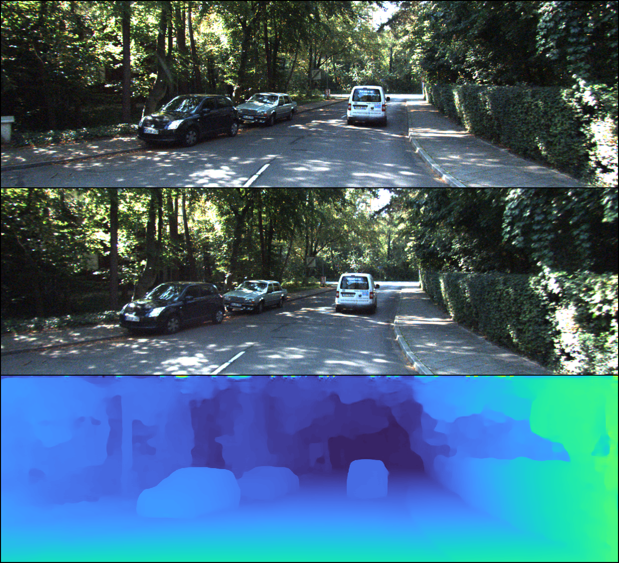
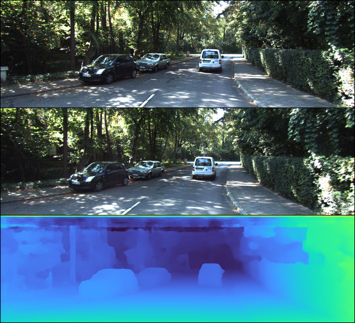
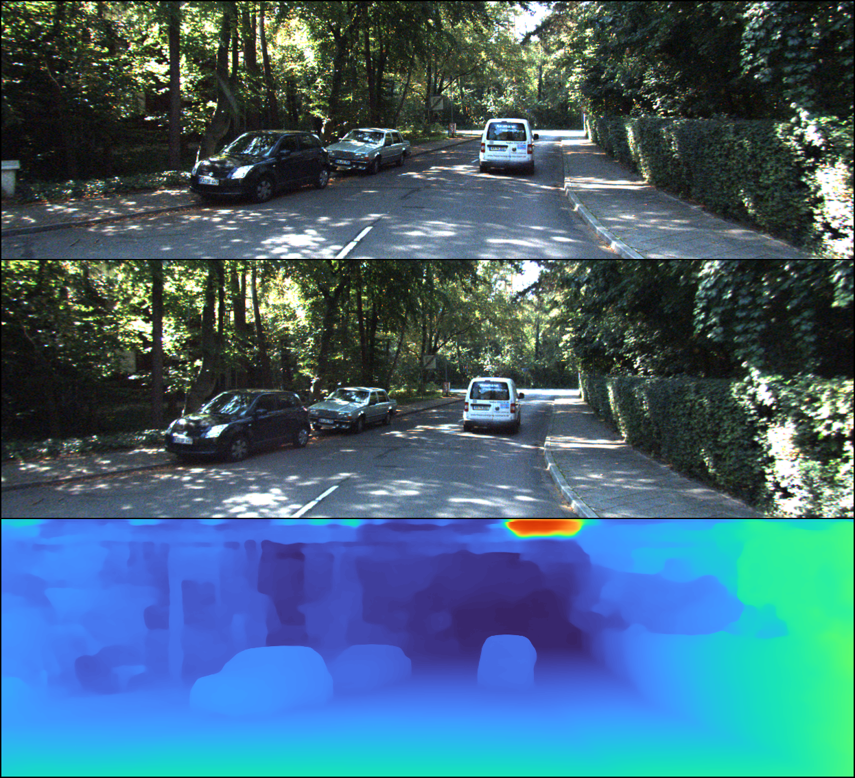
We notice that all these images have some artifacts at the top of the image (likely due to the fact that KITTI 2015 doesn’t provide point cloud cloud data for the upper portions of most images).
StereoNet Issues
Reflection
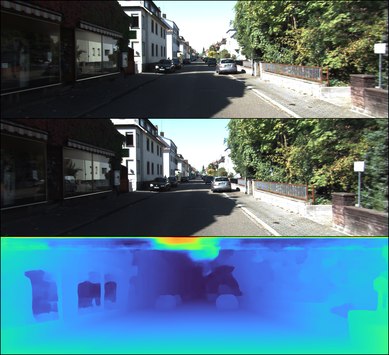
As mentioned in the original StereoNet paper, the StereoNet model struggles a bit with relections as its refinement network doesn’t have a good structure for solving the inpainting problem. As a window that has depth both behind it and at the window’s surface has ambiguous depth, but the loss is computed based on whatever the lidar reports, the model can score a bit lower on evaluation metrics for actually trying to report depth of objects behind the window surface. The authors mention that some of the models that perform better than theirs likely learn to paint over this surface (inpainting) and thus ignore the object behind the window glass. We can see in Figure 7 the model struggles with the reflections on the window of the store front.
Unlabeled Sky
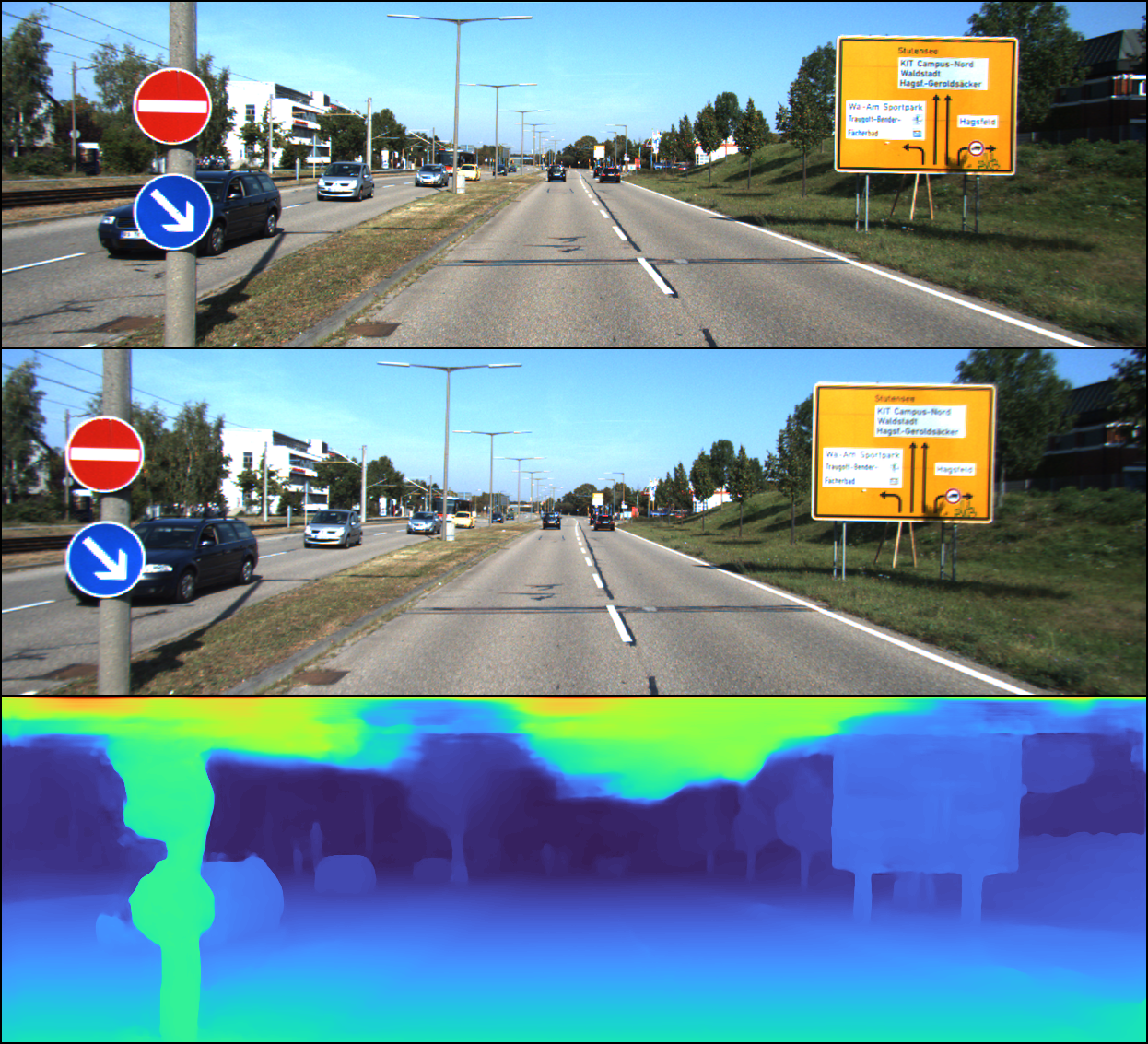
In the Kitti 2015 dataset, point clouds often only extend to the upper half of the image. We found that this could be problematic for learning the depth map for the sky as this is a fairly textureless region and thus many possible disparity values are valid. This makes the softmax over the cost volume have many equal value paths, and the model seems to learn to favor a lower disparity in these cases, creating many artifacts in the sky. The ideal way to fix this would be to augment the sky with additional data points (likely labeling the sky as close to infinity) so the refinement network could learn to treat the sky differently than the rest of the model. As attaining additional labeled data is difficult, we instead proposed a different solution using some of the features from HITNet in an attempt to solve this issue.
Rough Object Boundaries
We finally notice that some of our boundaries on objects in StereoNet are a bit bloblike and not as precise as one may expect. This is due to the model needing more training time on the refinement network and not an issue with the actual model design.
Experimental Contributions
NonSiamese StereoNet
When looking at the StereoNet Model we were somewhat curious what the effect of using a Siamese network had on the model, over training separate models for both left and right images. We surmised that there may be some differences in images depending on the side they were taken on and it might make sense to learn a different representation for each of these pieces of the network. As the feature refinement part of the network as well as the cost matrix are likely very similar in function, we only trained separate features for both model sizes. While this does effectively reduce by half our quantity of training data per weight in the feature generation of our network(as we are no longer training the weights per iteration on both the left and right images) we were hopeful it might result in a slight performance gain.
self.feature_extractor_left = [conv_3x3(3, 32, 2), ResBlock(32)]
self.feature_extractor_right = [conv_3x3(3, 32, 2), ResBlock(32)]
for _ in range(self.k - 1):
    self.feature_extractor_left += [conv_3x3(32, 32, 2), ResBlock(32)]
    self.feature_extractor_right += [conv_3x3(32, 32, 2), ResBlock(32)]
self.feature_extractor_left += [nn.Conv2d(32, 32, 3, 1, 1)]
self.feature_extractor_right += [nn.Conv2d(32, 32, 3, 1, 1)]

self.feature_extractor_left = nn.Sequential(*self.feature_extractor_left)
self.feature_extractor_right = nn.Sequential(*self.feature_extractor_right)
We quickly realized that this was not a good idea as the loss of the model went down much much more slowly and it became clear it wouldn’t converge to anything relevant very quickly. Reflecting on this once more, this does make some sense, as we likely want the main features of the left and right images to be the same, just with minor tweaks per model. It may make sense to finetune the Siamese network allowing each side to train separately using this logic, but due to a limitation on remaining Google cloud credits, we decided not to test this hypothesis and move on to other ideas.
Optimizer and Loss Function Tweaks
In the original StereoNet paper, and in the implementation we based ours off, the authors used RMSProp. We thought we could speed up the training process by choosing a different optimizer, so we changed it to Adam with $\lambda = 4\times10^{-4}$. The authors also make use of the robust loss function presented in [6] with \(\alpha = 1\) and \(c = 2\), which we found adjusting to $ \alpha=0.5 $ and $ c = 0.8 $ resulted in the model training a bit faster. Also, in the implementation of StereoNet we based our code off of, it used plain ReLU activation everywhere. This contradicts the original StereoNet paper, and in theory is more susceptible to vanishing gradients, so in our version we changed to LeakyReLU activation.
Model Structure
In StereoNet, after computing the 3D cost volume, the model filters it with 5 layers of 3D convolutions with kernel size 3. In theory, this should allow for learning to correct inaccuracies in the cost volume, but it also means that the model must learn to not lose the original cost volume features. We theorized that the model would train faster by placing 3D convolutions in ResNet blocks with shortcuts. In our results, we indeed see that the model trains much faster, achieving the same train accuracy in one quarter of the time, while attaining nearly the same validation accuracy.
Future Suggestions
Below are a couple suggestions that we considered when training, but weren’t able to actually experiment with as we ran out of Google Cloud Credits.
HITNet Initialization in FineTuning Loss Optimization of StereoNet Refinement
The main issue we noticed on training StereoNet on the Kitti 2015 dataset was its inability to identify the sky in the image as having infinite distance away from the cameras and instead predicting it was very close to the viewer. Although this is somewhat an issue of the dataset not labeling the sky making it difficult for the model to learn this feature we were hopeful that we could solve this problem in the edge detection (refinement) layer used in StereoNet. Our hope was that this refinement network could learn the position of the sky in the image and skew this value to have a small disparity (thus far away depth). In order to do this we took our already trained version of StereoNet and used the initialization model (with its already trained parameters from our training of HITNet) to add an additional loss to the refinement layer. As HITNet correctly classified the sky (and its initialization just gives a noisy version of correct classification), we hoped that adding this to our loss computation for StereoNet would bias the refinement layer to omit the sky from our final output.
Artificial Texture
Another idea we had for addressing the issue with the sky was adding an artificial texture to the images. By adding a series of dots on both images with a fixed disparity we could take the same idea from active stereo of the dot projection matrix and try to bias the disparities predicted for textureless regions. A downside of this approach is it would lead to an issue with potentially incorrect disparities on other regions with many pixels of same colors. This certainly isn’t a perfect solution, but performing this change and only altering the images above 80% of the height of the image would likely be sufficient to target a rough approximation of the sky region as the Kitti dataset is biased to include sky regions in this approximate area.
Useful Links
You can find a link to our final presentation, our presentation video, and a demo notebook of our results here.
Reference
[1] Zhuoran Shen, et al. “Efficient Attention: Attention with Linear Complexities.” Winter Conference on Applications of Computer Vision. 2021.
[2] Vladimir Tankovich, et al. “HITNet: Hierarchical Iterative Tile Refinement Network for Real-time Stereo Matching.” Conference on Computer Vision and Pattern Recognition. 2021.
[3] Jia-Ren Chang, et al. “Pyramid Stereo Matching Network.” Conference on Computer Vision and Pattern Recognition. 2018.
[4] Nikolai Smolyanskiy, et al. “On the Importance of Stereo for Accurate Depth Estimation: An Efficient Semi-Supervised Deep Neural Network Approach.” Conference on Computer Vision and Pattern Recognition. 2018.
[5] Olaf Ronneberger, et al. “U-Net: Convolutional Networks for Biomedical Image Segmentation” Conference on Computer Vision and Pattern Recognition. 2015.
[6] Barron, J.T. “A more general robust loss function.” Conference on Computer Vision and Pattern Recognition. 2017.
[7] zjjMaiMai on GitHub. TinyHITNet GitHub. 2021.