NeX novel view synthesis
Novel view synthesis aims to generate a visual scene representation from just a sparse set of images and has a wide variety of uses in VR/AR. In this blog, we will explore a new approach to this problem called NeX.
- Introduction
- Spotlight Video
- MPI
- NeRF
- A New Way of Modeling Color
- Multilayer Perceptrons
- Algorithm
- Implementation
- Demo
- Reference
- Code Repository
Introduction
We will explore NeX [1], a new method of novel view synthesis that uses enhanced multiplane image (MPI) [2] techniques to produce view-dependent effects in real-time.
Spotlight Video

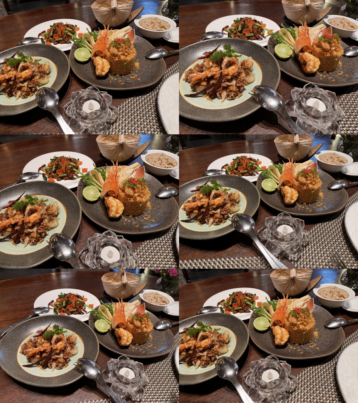
Sparse images to smooth video [1].
MPI
NeX aims to improve upon a previous approach to view synthesis called multiplane image (MPI). MPI uses deep neural networks to extrapolate new views with just two stereo input images. The network takes in as input the two input images as well as camera parameters and infers a global scene representation. The scene is represented as a set of planes, each of which represents an RGB color image and \(\alpha\)/transparency map at a certain depth. In each layer the \(\alpha\) map is used to occlude certain pixels based on the depth. Then, these planes can then be used to synthesize novel views using homography and composition functions.
While MPI is a more effective solution to view synthesis than previous methods, it still had some issues. Namely, the RGB\(\alpha\) representation works best on diffuse surfaces and struggles to capture view-dependent effects like reflections and specular highlights. MPI also suffers from expensive inference which prohibit real-time rendering.
NeRF
NeRF [3] is one of the state of the art methods proposed to solve this problem of capturing view-dependent effects. It takes in as input the 3D spacial location as well as viewing direction and uses a deep fully connected network to directly learn colors and view-dependent raidance. Although NeRF successfully captures reflections and specular highlights well, it, like MPI, suffers from being unable to be rendered in real-time.
A New Way of Modeling Color
NeX solves this problem by parameterizing each color value in the MPI as a function of the viewing angle instead of storing color as a static value. This function is approximated as a linear combination of learnable spherical basis functions: \(C^p(v) = k^p_0 + \sum_{n=1}^{N}k^p_nH_n(v)\) where \(k^p_n\) for pixel \(p\) is the RGB coefficient/reflectence parameters for the \(N\) basis functions denoted by \(H_n(v)\). Two separate Multilayer perceptrons (MLP) are used to optimize the parameters and basis functions.
Multilayer Perceptrons
The first MLP predicts per-pixel parameters given the pixel location:
\[F_\theta : (x) \rightarrow (\alpha,k_1,k_2,...,k_N)\]where \(x = (x, y, d)\) contains the location information of the pixel \((x, y)\) at depth \(d\). The second MLP is used for predicting all global basis functions given the viewing angle. This second MLP is kept separate to ensure that the basis functions are not functions of pixel location and is modeled by:
\[G_\phi: (v) \rightarrow (H_1,H_2,...,H_N)\]where \(v\) is the normalized viewing direction.
It should be noted that for \(F_\theta\), the first coefficient, \(k_0\), is not learned but instead stored explicitiy so as to keep a “base color” for each pixel and help retain finer details while also reducing computation cost. Another optimization done is sharing coefficients across multiple planes instead of computing different coefficients for each individual pixel, which results in significant speed gain without compromising visual quality. To optimize the model, the two MLP’s are evaluated to generate an output image which is then compared with a ground truth image at the same view. The loss is given as follows:
where \(\hat{I_i}\) is the reconstructed image and \(I_i\) is the ground truth image.
Algorithm
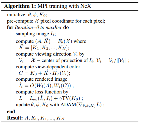
Fig 1. NeX training algorithm [1].
To summarize, first compute pixel location information for each pixel and for each iteration, compute \(\alpha\) and pixel parameters \(\vec{K}\) with \(F_\theta\). Then, compute the viewing angle \(v\) and evaluate \(G_\phi\) to get the basis functions \(\vec{H}_\phi(v)\). Get the color functions \(C\) via linear combination of the \(\vec{K}\) and \(\vec{H}_\phi(v)\) and compose the image using \(\alpha\) and \(C\). Finally, compute the loss and optimize.
Implementation
First the images are preprocessed with COLMAP [4] structure-from-motion algorithm in order to calibrate the images. COLMAP is a tool that allows us to establish structure from motion. In other words, using some conventional computer vision algorithms (including SIFT), it is able to identify feature points in each image, match feature points between different images, produce a comprehensive mapping of feature points to point clouds in 3D-space, then export this mapping.
Below, you can see an animation we generated from the rendered point-cloud in COLMAP.
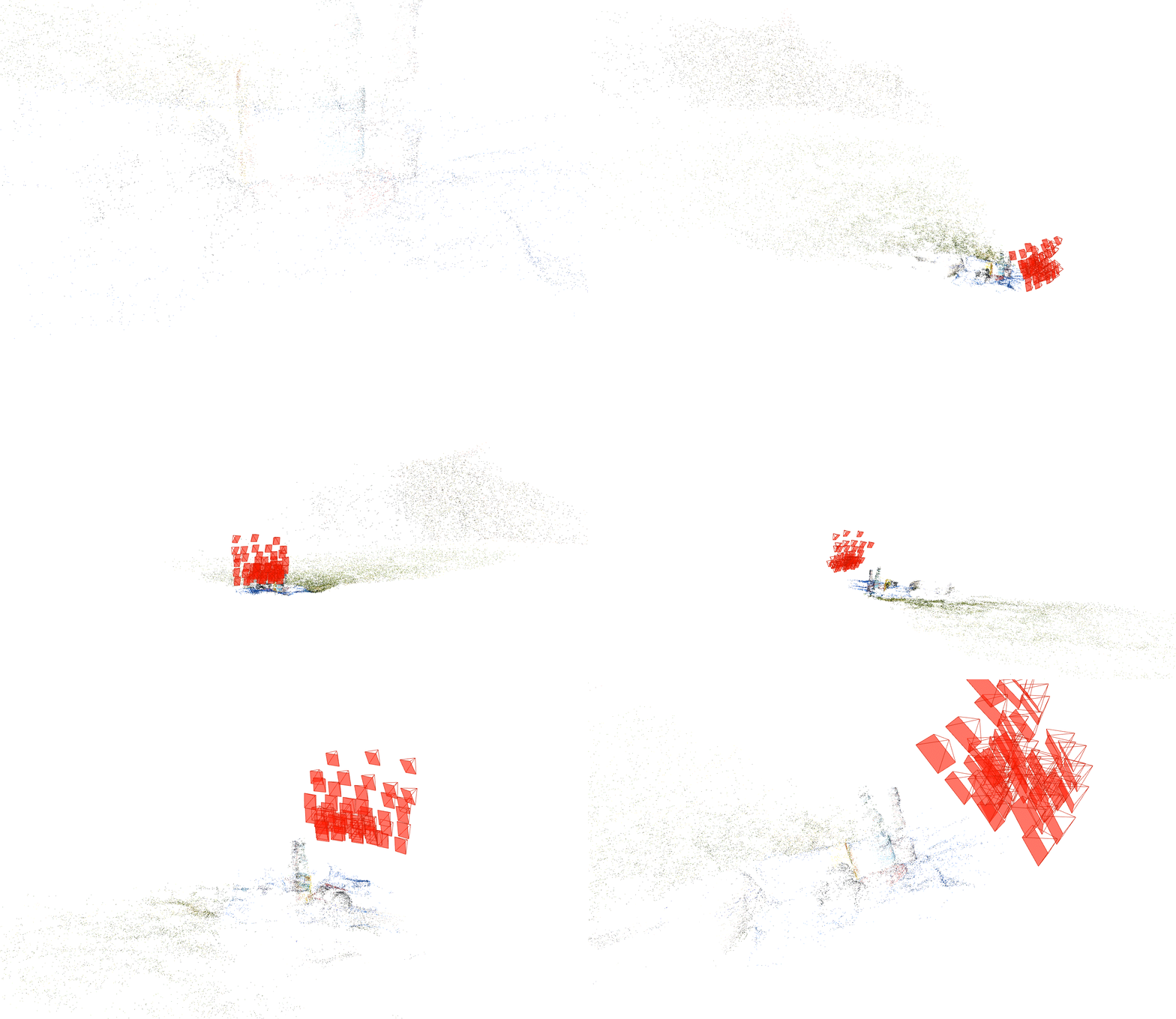 Fig 2. Point-cloud representation of our scene.
After COLMAP, we can run the first MLP
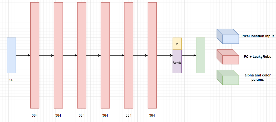
Fig 3. First MLP architecture.
For computing \(\alpha\) and pixel parameters with \(F_\theta\), the pixel location input \((x, y)\) takes 40 dimensions while the depth d takes 16 dimensions, totalling the input to 56 dimensions. The network consists of 6 fully connected layers with LeakyReLU activation, each with 384 nodes. The final output consists of \(\alpha\), which uses sigmoid activation, and \(\vec{K}\), which uses \(tanh\) activation.
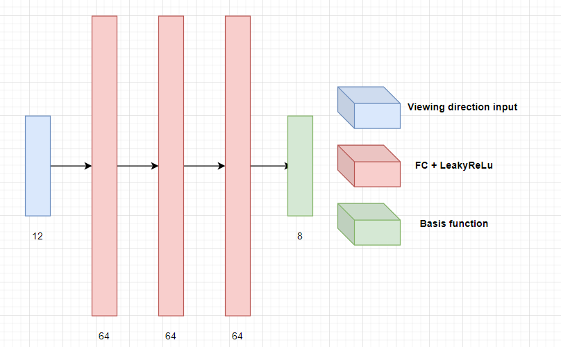
Fig 4. Second MLP architecture.
\(G_\phi\) takes in as input a 12 dimension input for viewing direction and consists of 3 fully connected layers with LeakyReLU activation, each with 64 nodes. The 8-dimensional output are the basis functions \(\vec{H}_\phi(v)\).
Demo
Colab Demo (Based on code from original authors)
Our goal for the demo was to produce a working NeX view synthesis model, based on a dataset of our own images, including training our own model and producing a final output video.
This process can be broken into several steps, including:
- Creating input data
- Preprocessing images
- Building structure-from-motion using COLMAP
- Adapting dataset for NeX
- Training NeX model
Collecting input images
We decided to try to create a challenging scene, including several reflective objects including a few glass bottles of liquid, a shiny foil snack wrapper, and a camera with a reflective front lens element. A video showing the real-world view (perhaps the ultimate “ground truth”) is available here:
We tested several formats of image collection, including taking images in a grid vs. randomly, and taking images all in the same orientation vs. taking images all aligned towards the center of the scene, but found no significant differences in our result.
Due to the limitations of our Colab credit, we found that we could not efficiently train the model on output images larger than 600 pixels in width, so before training, we resized all of our input images to be 800x600.
Training NeX Model
We trained several NeX models to learn more about the process. First, we used the readily available “sushi” dataset, trained for 40 epochs:
We used this as the goal for the quality we hoped to achieve with our own dataset.
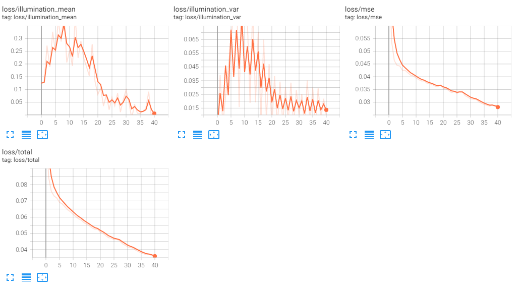
Next, we used a small sample of images from the various images we collected, using 20 images out of the total 60 we collected, and also trained for 40 epochs:
As you can see, although there is some structure present (note the yellow from the drink box, the black of the camera, and the blue of the blanket), this is nowhere near the quality of the provided sushi dataset. Of course, this may be due to the quality of our input data. Looking at the reported loss (below) and comparing to the sushi dataset, we saw that the loss was still quite high, but decreasing steadily, so we decided to train for another 360 epochs, for a total of 400.
Here is the result of the 20-image dataset, trained for 400 epochs:
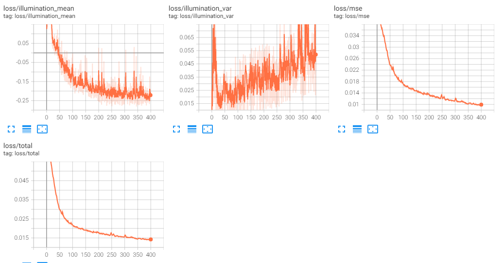
As you can see, this is quite promising. The quality has improved dramatically, and we are starting to see finer details on the various objects. We can expect that as we approach 4000 epochs, the number of epochs that the original model was trained for, that we may start to see much better details.
We hypothesize that the reason why our dataset is taking so much longer to train versus the sushi dataset, is that the sushi dataset is relatively simple compared to ours. We have many different textures and objects in the scene, including a field of grass in the background, which contributes to a very complex point cloud for NeX to process. It seems that the neural network is struggling with this scene (as we intended), although more testing is needed to see exactly why.
Although we could have chosen to continue training for all 4000 epochs, we decided to take a different approach, and use all 60 images to produce another dataset, trained for 400 epochs.
Here we see that even though we trained with a much more robust dataset, with much more information, and trained for 400 epochs, this result is even worse than our initial 20-image dataset for 40 epochs. What could have gone wrong?
Looking at the loss, it seems like this model is learning even slower:
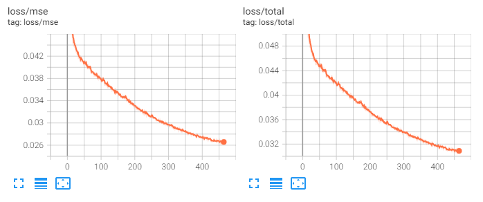
Although it is still making progress, it seems that the 60-image dataset will require training for far longer to produce acceptable results.
Demo conclusion
We ran into a few issues while attempting to create our own demo view/dataset. For one, it was challenging to get COLMAP to work with CUDA in the Colab environment, which is why we suspect the original team may have omitted COLMAP CUDA support originally. Additionally, it was difficult to understand and use the COLMAP tool, and to convert the COLMAP export files into the format that the NeX training code required. Finally, we learned that more input images doesn’t always produce better results.
For future exploration, a few interesting areas might be what the optimal number of input view images are, the performance of the model when the objects of interest are varying distances from the camera, and of course, alternative MLP architectures that may improve both the training and evaluation performance overall.
Reference
[1] Wizadwongsa, Suttisak, et al. “NeX: Real-time View Synthesis with Neural Basis Expansion” arXiv preprint arXiv:2103.05606. (2021).
[2] Zhou, Tinghui, et al. “Stereo Magnification: Learning view synthesis using multiplane images” arXiv preprint arXiv:1805.09817 (2018).
[3] Ben Mildenhall, et al. “NeRF: Representing Scenes as Neural Radiance Fields for View Synthesis” Proceedings of ECCV conference (2020).
[4] Johannes Lutz Schonberger and Jan-Michael Frahm. “Structure-from-motion revisited.” In Conference on Computer Vision and Pattern Recognition (CVPR), 2016.
Code Repository
[1] NeX Wizadwongsa, Suttisak, et al.