CLIP and Some Applicatios
CLIP (Contrastive Language-Image Pre-training) is a neural network model developed by OpenAI that combines the strengths of both computer vision and natural language processing to improve image recognition and object classification. CLIP has been shown to achieve state-of-the-art results on a wide range of image recognition benchmarks, and it has been used in various applications such as image captioning and image search. I found an open-source SimpleCLIP model online and conducted some experiments to reconstruct the model. Using ideas and methods from some papers, I attempted to address its overfitting issue.
- Contrastive Learning
- Main Content in CLIP Paper
- Implementaion of CLIP
- Experiments of hyperparameters
- Result
- Review
- Reference
Contrastive Learning
MoCO And SimClR
Unsupervised representation learning has shown great success in natural language processing (NLP), but supervised pre-training remains dominant in the visual field. Despite this, there is a lot of promising unsupervised work in the visual field, although it tends to perform worse than supervised models. The authors suggest that this may be due to the vastly different signal space in the two fields.
In NLP, the signal space is discrete, represented by words or root affixes. This makes it easy to create tokenized dictionaries and perform unsupervised learning. However, in the visual field, the signal is continuous and high-dimensional, lacking strong semantic information like words. This makes it difficult to create a dictionary, as the condensation is not concise.
Here is a simple flow chart:
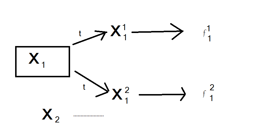
Fig.
To overcome this challenge, the authors propose a dynamic dictionary method for unsupervised representation learning in the visual field. The method involves selecting a random image from a dataset and performing different transformations on it to obtain positive sample pairs. The remaining images in the dataset serve as negative samples. The samples are then passed through an encoder to obtain feature outputs, and contrastive learning is used to make the positive sample pair features as similar as possible while keeping the negative sample features far away from the positive sample features in the feature space.
The dynamic dictionary is created by treating the features obtained from the encoder as entries in a dictionary. The goal is to train the encoder to perform dictionary lookups, with the encoded query (feature output) as similar as possible to the feature of the matching key (positive sample feature). The dictionary must be large and consistent during training to sample from the continuous high-dimensional visual space and represent rich visual features.
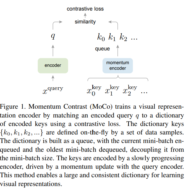
Fig 1. Momentum Contrast for Unsupervised Visual Representation Learning [3].
A small dictionary could lead to a shortcut solution, which prevents the pre-trained model from generalizing well. Consistency is also important, as keys in the dictionary should be generated using the same or similar encoders to ensure that comparisons are as consistent as possible. This prevents the model from learning shortcut solutions that do not contain the same semantic information.
The objective function for comparative learning should meet certain requirements. Firstly, when the query q is similar to the only positive sample k plus, the loss value should be relatively low. Secondly, even when the query q is dissimilar to all other keys, the loss value should still be low. If these requirements are met, it indicates that the model is almost fully trained. Naturally, we want the loss value of the objective function to be as low as possible so that we do not need to update the model.
Conversely, if the query q is dissimilar to the positive sample key plus or if the query q is similar to the keys that should have been negative samples, then the loss value of the objective function should be as large as possible. This is done to penalize the model and prompt it to quickly update its parameters. The InfoNCE contrastive learning function was adopted for this purpose.
\[\label{eq:loss} \mathcal{L}_{\mathrm{N}}=-\underset{X}{\mathbb{E}}\left[\log \frac{f_{k}\left(x_{t+k}, c_{t}\right)}{\sum_{x_{j} \in X} f_{k}\left(x_{j}, c_{t}\right)}\right],\]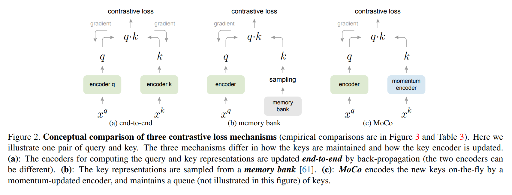
Fig 1. Momentum Contrast for Unsupervised Visual Representation Learning [3].
Why we need the large batch size?
In the Figure, the author also wrote that the encoders q and k can be different networks but before, many works used the same network. For the sake of simplicity, in MoCo’s experiment, the encoder q and k are the same model, which is a Res 50. Because both positive and negative samples come from the same Mini-batch, it means that \(x_q\) and \(x_k\) here are all from the same batch. He can get the characteristics of all samples by doing one forward, and these samples are highly consistent. The limitation lies in the size of the dictionary, because the size of the dictionary is equivalent to the size of the mini-batch size in the end-to-end learning framework. Then if we want a large dictionary with tens of thousands of keys, it means that the mini-batch size must also be tens of thousands, which is very difficult.(The SimClR uses the end-to-end learning framework.)
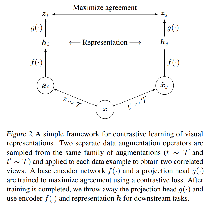
Fig 2. A Simple Framework for Contrastive Learning of Visual Representations [2].
I introduced these concepts first to illustrate something about the idea in experiments with small data and small batch sizes.
Main Content in CLIP Paper
Concepts explanation in CLIP idea
Contrastive Learning: This is a method used to teach a model to recognize the similarities and differences between different types of data. In the case of CLIP, the model is trained on pairs of images and their associated textual descriptions. During training, the model learns to identify which images and descriptions are related and which are not. This helps the model learn to understand the relationships between different types of data.
Multi-Task Learning: Multi-task learning is a technique that allows a model to learn multiple tasks simultaneously. In the case of CLIP, the model is trained to perform multiple tasks, such as image classification, object detection, and natural language processing. This approach allows the model to learn to recognize patterns in both images and text, and to make connections between them.
Zero-Shot Learning: Zero-shot learning is a technique used to teach a model to recognize objects or concepts that it has not been explicitly trained on. In the case of CLIP, the model is trained on a large dataset of images and their associated textual descriptions. This allows the model to learn to recognize a wide range of objects and concepts, even if it has never seen them before.
Pre-Training on Large Datasets: CLIP is pre-trained on a large dataset of images and their associated textual descriptions. This pre-training allows the model to learn to recognize a wide range of objects and concepts, and to understand the relationships between them. This pre-training is essential to the model’s ability to perform well on a wide range of tasks. Overall, these approaches work together to create a powerful model that can recognize a wide range of objects and concepts, and understand the relationships between them, using both images and text.
The main method
The key to CLIP’s ability to perform zero-shot learning is its use of a shared embedding space that maps both images and text into a common feature space. During training, CLIP is trained to associate images and their corresponding text descriptions with similar feature vectors in the embedding space, and to associate dissimilar pairs with dissimilar feature vectors. This allows CLIP to learn to recognize and differentiate between a wide variety of objects and concepts based on their textual descriptions, even if it has not been explicitly trained on them. To perform zero-shot learning, CLIP takes a new textual description as input and maps it into the embedding space to obtain a feature vector. It then searches for the image in the dataset that has the most similar feature vector to the input description. The image that best matches the input description is returned as the model’s prediction. CLIP is able to perform zero-shot learning on a wide range of objects and concepts, including ones that are rare, obscure, or previously unseen, as long as they can be described using natural language. This makes it a powerful tool for a wide range of applications, including computer vision, natural language processing, and other areas where it is difficult or impractical to obtain large datasets of labeled examples.
Model
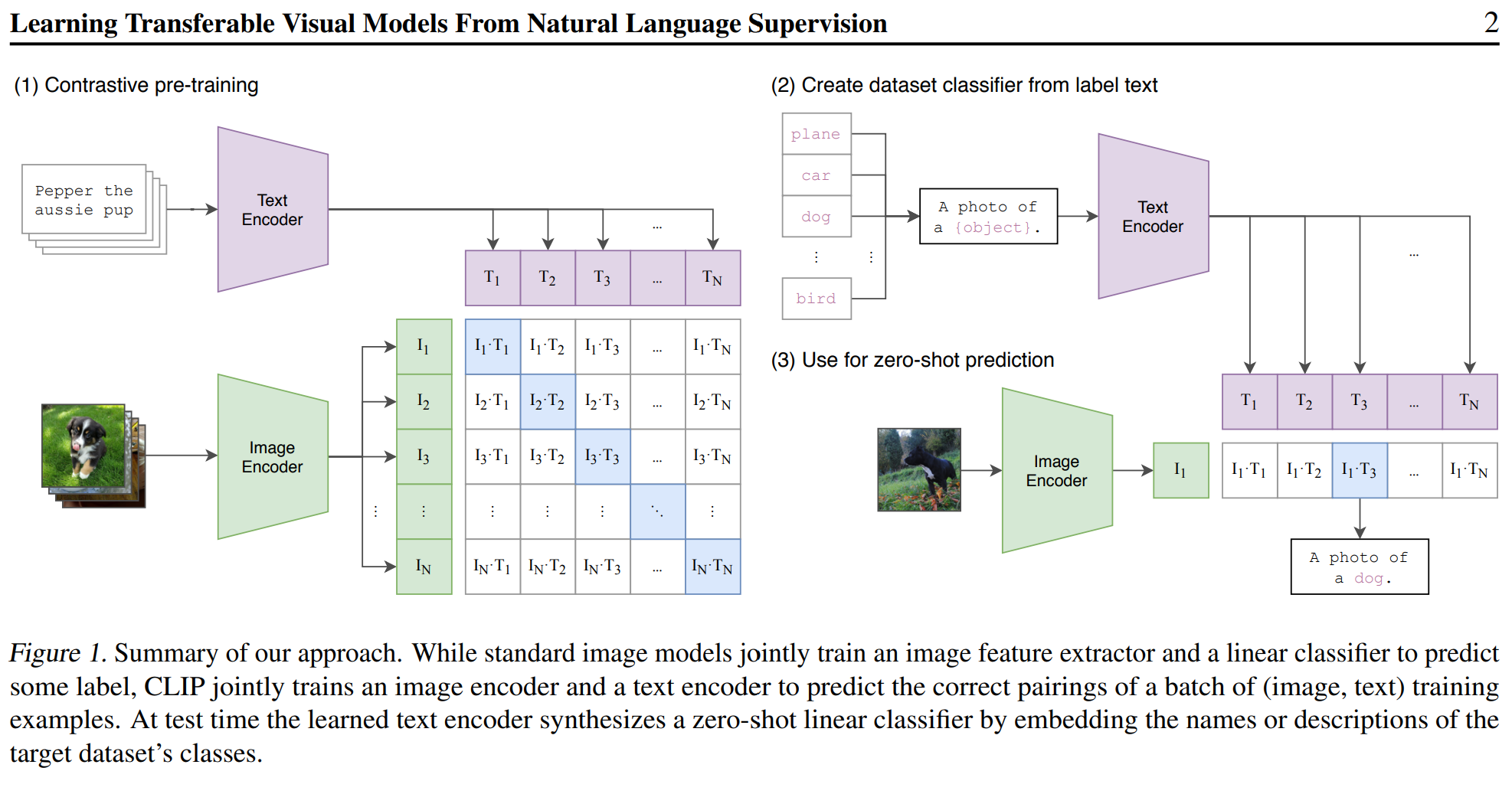
Fig 3. Learning Transferable Visual Models From Natural Language Supervision [1].
Explanation
The figure shows that while standard image models train an image feature extractor and a linear classifier to predict some label, the proposed approach, CLIP, jointly trains an image encoder and a text encoder to predict the correct pairings of a batch of (image, text) training examples.
The image encoder is a deep neural network that takes an image as input and produces a feature vector as output. The text encoder is a deep neural network that takes a text description as input and produces a feature vector as output. The two feature vectors are then compared to determine if the image and text description are a correct pairing.
At test time, the learned text encoder is used to synthesize a zero-shot linear classifier by embedding the names or descriptions of the target dataset’s classes. This means that the text encoder is used to generate a feature vector for each class in the target dataset, and these feature vectors are then used to create a linear classifier that can be used to classify images without any additional training.
Another attetion
The phrase “A photo of” can be considered as a visual prompt or context that is used to guide the encoding of the following text into an image embedding. By including this prompt, the CLIP model is able to understand that the text following the prompt refers to an image or a visual concept, and can use this information to generate a more accurate image embedding.
For example, if the text following the prompt is “a cat sleeping on a windowsill”, the CLIP model will use the prompt to generate an image embedding that represents the concept of a cat sleeping on a windowsill. This is done by encoding both the visual features of the cat and the windowsill, as well as the semantic meaning of the text, into a single vector representation.
By including visual prompts such as “A photo of”, the CLIP model is able to better understand the relationship between text and images, which allows it to perform tasks such as image classification and visual question answering with greater accuracy and efficiency.
Pseudocode in paper
# image_encoder - ResNet or Vision Transformer
# text_encoder - CBOW or Text Transformer
# I[n, h, w, c] - minibatch of aligned images
# T[n, l] - minibatch of aligned texts
# W_i[d_i, d_e] - learned proj of image to embed
# W_t[d_t, d_e] - learned proj of text to embed
# t - learned temperature parameter

# extract feature representations of each modality
I_f = image_encoder(I) #[n, d_i]
T_f = text_encoder(T) #[n, d_t]

# joint multimodal embedding [n, d_e]
I_e = l2_normalize(np.dot(I_f, W_i), axis=1)
T_e = l2_normalize(np.dot(T_f, W_t), axis=1)
# scaled pairwise cosine similarities [n, n]
logits = np.dot(I_e, T_e.T) * np.exp(t)

# symmetric loss function
labels = np.arange(n)
loss_i = cross_entropy_loss(logits, labels, axis=0)
loss_t = cross_entropy_loss(logits, labels, axis=1)
loss = (loss_i + loss_t)/2

Numpy-like pseudocode for the core of an implementation of CLIP.
Results of the paper
- The results of this paper show that the proposed approach is an efficient and scalable way to learn state-of-the art (SOTA) representations from scratch on large datasets.
- After pre-training with this method, natural language can be used to reference learned visual concepts or describe new ones without needing additional labeled data - enabling zero shot transfer of the model onto downstream tasks such as OCR, action recognition in videos etc..
- It was benchmarked against over 30 existing computer vision datasets and it showed non trivial transfers across most tasks while being competitive with fully supervised baselines without any dataset specific training required.
- In particular, we matched the accuracy of a ResNet50 trained on ImageNet using only text descriptions instead of 1.28 million images for training purposes
Implementaion of CLIP
The whole colab code would post in ref. The following are some explanations about the process.
dataset
Flicker Dataset(e.g. Flicker8k_Dataset):
| image | caption | id | |
|---|---|---|---|
| 0 | 1000268201_693b08cb0e.jpg | A child in a pink dress is climbing up a set o… | 0 |
| 1 | 1000268201_693b08cb0e.jpg | A girl going into a wooden building . | 0 |
Hyperparameters
class CFG:
    debug = False
    image_path = image_path
    captions_path = captions_path
    batch_size = 32
    num_workers = 2
    head_lr = 1e-3
    image_encoder_lr = 1e-4
    text_encoder_lr = 1e-5
    weight_decay = 1e-3
    patience = 1
    factor = 0.8
    epochs = 4
    device = torch.device("cuda" if torch.cuda.is_available() else "cpu")

    model_name = 'resnet50'
    image_embedding = 2048
    text_encoder_model = "distilbert-base-uncased"
    text_embedding = 768
    text_tokenizer = "distilbert-base-uncased"
    max_length = 200

    pretrained = True # for both image encoder and text encoder
    trainable = True # for both image encoder and text encoder
    temperature = 1.0

    # image size
    size = 224

    # for projection head; used for both image and text encoders
    num_projection_layers = 1
    projection_dim = 256
    dropout = 0.1
Clip Model
class CLIPModel(nn.Module):
    def __init__(
        self,
        temperature=CFG.temperature,
        image_embedding=CFG.image_embedding,
        text_embedding=CFG.text_embedding,
    ):
        super().__init__()
        self.image_encoder = ImageEncoder()
        self.text_encoder = TextEncoder()
        self.image_projection = ProjectionHead(embedding_dim=image_embedding)
        self.text_projection = ProjectionHead(embedding_dim=text_embedding)
        self.temperature = temperature

    def forward(self, batch):
        # Getting Image and Text Features
        image_features = self.image_encoder(batch["image"])
        text_features = self.text_encoder(
            input_ids=batch["input_ids"], attention_mask=batch["attention_mask"]
        )
        # Getting Image and Text Embeddings (with same dimension)
        image_embeddings = self.image_projection(image_features)
        text_embeddings = self.text_projection(text_features)

        # Calculating the Loss
        logits = (text_embeddings @ image_embeddings.T) / self.temperature
        images_similarity = image_embeddings @ image_embeddings.T
        texts_similarity = text_embeddings @ text_embeddings.T
        targets = F.softmax(
            (images_similarity + texts_similarity) / 2 * self.temperature, dim=-1
        )
        texts_loss = cross_entropy(logits, targets, reduction='none')
        images_loss = cross_entropy(logits.T, targets.T, reduction='none')
        loss =  (images_loss + texts_loss) / 2.0 # shape: (batch_size)
        return loss.mean()


def cross_entropy(preds, targets, reduction='none'):
    log_softmax = nn.LogSoftmax(dim=-1)
    loss = (-targets * log_softmax(preds)).sum(1)
    if reduction == "none":
        return loss
    elif reduction == "mean":
        return loss.mean()
The code measures similarility of two groups of vectors (two matrices) are to each other with dot product (@ operator in PyTorch does the dot product or matrix multiplication in this case). To be able to multiply these two matrices together, it transposes the second one, and get a matrix with shape (batch_size, batch_size) which we will call logits. (temperature is equal to 1.0, but it will be learnable later.).(In clip, they use cross entropy as loss function instead of InfoNCE.) ProjectionHead is smiliar to the SimCLR picture above.
Experiments of hyperparameters
Clip trains each model for 32 epochs at which point transfer performance begins to plateau due to overfitting[1]. In my case, it’s easier to overfit 30k datasets.
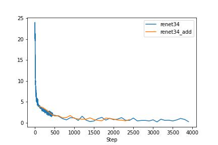
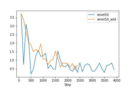
baseline of resnet50 and resnet34
Due to some GCP network reasons, I lost some train loss data. But Vaild loss is completely preserved. In the baseline, clip with resnet50 rans for 13 epchos and clip with resnet34 rans for 15 epchos.
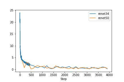
The networks are so powerful so that it overfitting to the small dataset.
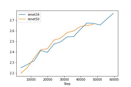
prompt before the photo caption
| image | caption_number | id | caption |
|---|---|---|---|
| 0 | 1000092795.jpg | 0 | This image shows two young guys with shaggy hair looking at their hands while hanging out in the yard. |
| 1 | 1000092795.jpg | 1 | This image shows two young, White males are outside near many bushes. |
| 2 | 1000092795.jpg | 2 | This image shows two men in green shirts are standing in a yard. |
| 3 | 1000092795.jpg | 3 | This image shows a man in a blue shirt standing in a garden. |
| 4 | 1000092795.jpg | 4 | This image shows two friends enjoy time spent together. |
Clip with resnet50 rans for 3 epchos and clip with resnet34 rans for 3 epchos. Compare with baseline
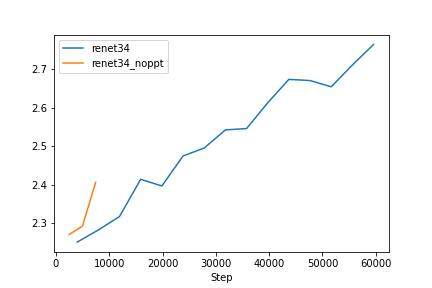
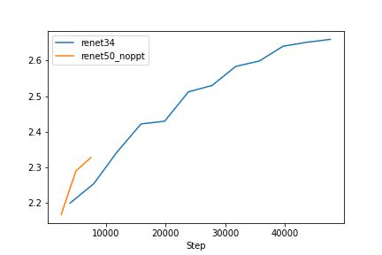
We can see that the prompt before the caption makes the model trains easier. In the next experiements, I will use the catption with the prompt. As the test loss graph shows, we can see that the text encoder is affecting the overfitting model. Therefore, I have decided to freeze the text encoder. Since I downgraded the image encoder that smaller than the text encoder model, it is reasonable to freeze the powerful text encoder or make the encoder learning rate small.
Overfitting
The simple Clip with resnet50 and one with resnet34 are so powerful,so I choose the restnet18. But the original resnet18 are also powerful.
Basic idea
As we learn in class, There are methods helpful to overfit: Dropout, weight decay, augmentation.
Idea from FLIP and MAE
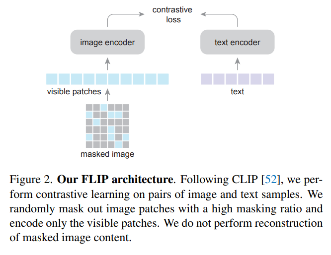
Fig 4. Scaling Language-Image Pre-training via Masking [4]. In the FLIP paper, they adopt the Vision Transformer (ViT) as the image encoder, so I choose to mask picture.
About FLIP:
- FLIP don’t use the MAE entire structure since they find it doesn’t improve the performance.
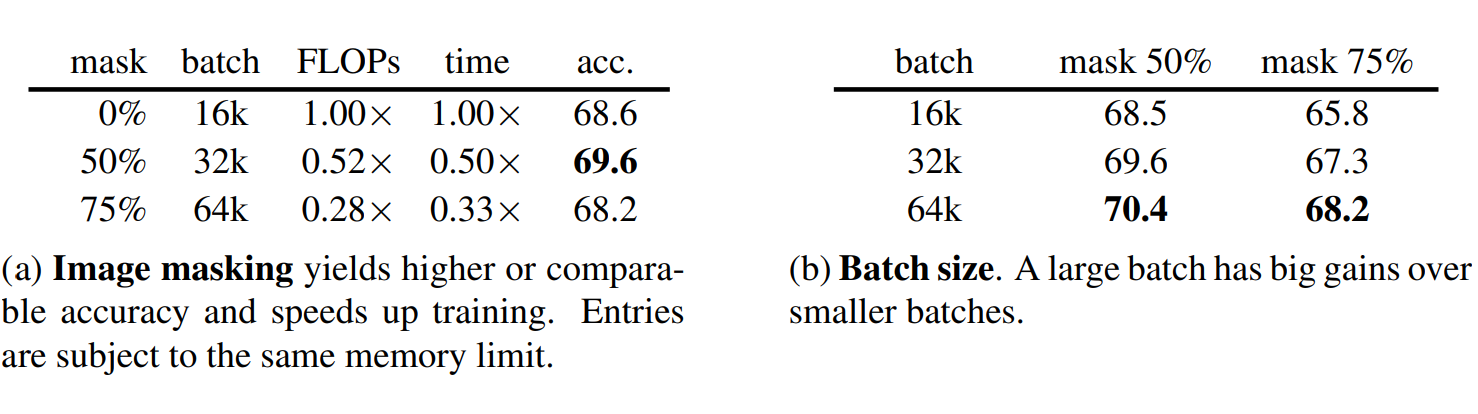
Fig 4. Scaling Language-Image Pre-training via Masking [4].
- It’s a little tricky that the reason of 50% mask has better score because of fast speed so that it trains larger datasize.
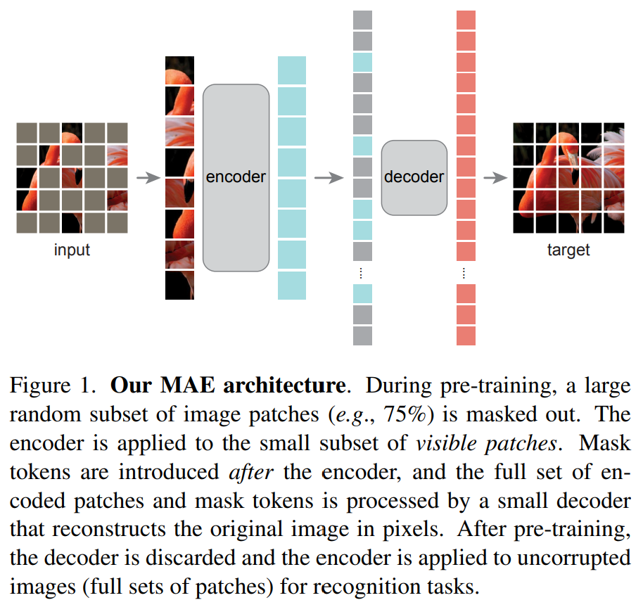
Like masking the encoder in MAE, I change the drop out of the projection of the Image Encoder. The methods are different, but that is the idea comes from.
Idea from MoCo
Since I have alrealy talk about the MoCo paper, I am not talking about it too much. I would change the batch size. I expect to see the perfomence better, since the larger batch size would make the dictionary larger.
Rebuild the simple model
The dataloader, model, and fine-tuning processes have all been rebuilt, but I have only introduced changes to the structure of some important modules. All of the code is in Colab.
Augmentation
def get_transforms(mode="train"):
    if mode == "train":
        return A.Compose(
            [
                A.PadIfNeeded(min_height=CFG.size, min_width=CFG.size),
                A.RandomCrop(width=CFG.size, height=CFG.size),
                A.HorizontalFlip(p=0.5),
                A.RandomBrightnessContrast(p=0.2),
                A.Normalize(max_pixel_value=255.0, always_apply=True),
                #A.CoarseDropout(max_holes=8, max_height=16, max_width=16, p=1.0),
                A.CoarseDropout(max_holes=16, max_height=32, max_width=32,  min_holes=8, p=1.0),

            ]
        )
    else:
        return A.Compose(
            [
                A.Resize(CFG.size, CFG.size, always_apply=True),
                A.Normalize(max_pixel_value=255.0, always_apply=True),
            ]
        )
Augmentation: RandomCrop, HorizontalFlip, RandomBrightnessContrast, CoarseDropout(Mask photos randomly).
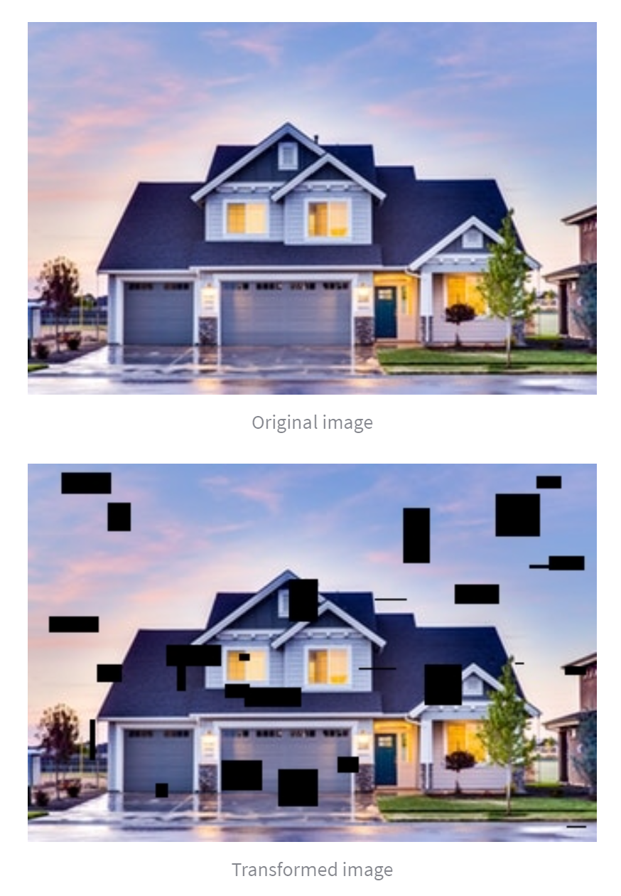
Fig 5. demo of CoarseDropout in https://demo.albumentations.ai/ .
Dropout_Image_encoder_Projection
class ProjectionHeadImage(nn.Module):
    def __init__(
        self,
        embedding_dim,
        projection_dim=CFG.projection_dim,
        dropout=CFG.dropout_Image #give the special hyperparameters
    ):
        super().__init__()
        self.projection = nn.Linear(embedding_dim, projection_dim)
        self.gelu = nn.GELU()
        self.fc = nn.Linear(projection_dim, projection_dim)
        self.dropout = nn.Dropout(dropout)
        self.layer_norm = nn.LayerNorm(projection_dim)

    def forward(self, x):
        projected = self.projection(x)
        x = self.gelu(projected)
        x = self.fc(x)
        x = self.dropout(x)
        x = x + projected
        x = self.layer_norm(x)
        return x
I add the ProjectionHeadImage in CLIP model to control the drop out of projection for image embedding. Due to the limited size of the GPU, I have to freeze the text encoder so that a larger batch size can be used. This experiment can be seen as using image encoding to learn text encoding, similar to distillation.
Result
Best average vaild loss(16 epochs)
| proption\batch size | 256 | 128 | 64 |
|---|---|---|---|
| 0.4 small mask | 3.49 | * | * |
| 0.4 large mask | 3.48 | * | * |
| 0.8 small mask | 3.40 | * | * |
| 0.8 large mask | 3.38 | 2.96 | 2.59 |
(20% dataset is test, small mask: 0.04. large mask 0.32.) Loss Curves for the follwing tensorboard link:tensorboard,tensorboard,tensorboard,tensorboard,tensorboard.
Discussion
From a masking perspective, it can be observed that suitable masks can improve the impact on the results, whether it is in 40% of the data or in 80% of the data. It can be said that this type of image data augmentation is effective in small data, which is consistent with the trend revealed in Flip. However, excessively large masks can also have an impact. For example, if we erase certain features from an image, but these features are reflected in the text code, it may affect the training results.
From the perspective of a larger batch size, it can be observed in this experiment that a larger batch size does not necessarily lead to better results, which goes against my original intention.
Why doesn’t this experiment follow the theory of Moco where larger batch sizes result in better training results? These are some reasons I can think of. First, the data in CLIP is very large, and training a large model with several hundred million data may require a larger batch size. However, in this experiment with a small model training on 30k data, a larger batch size is not suitable. Second, when using a larger batch size, it is often necessary to scale the learning rate accordingly to avoid overshooting the optimal solution. If the learning rate is not scaled correctly, the optimization can become unstable and lead to a higher loss. In particular, when using AdamW, it is important to ensure that the weight decay rate is also scaled accordingly to maintain the balance between the gradient updates and the weight decay.
Inference
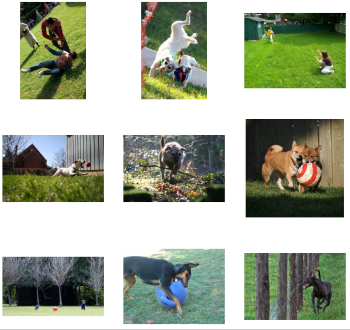
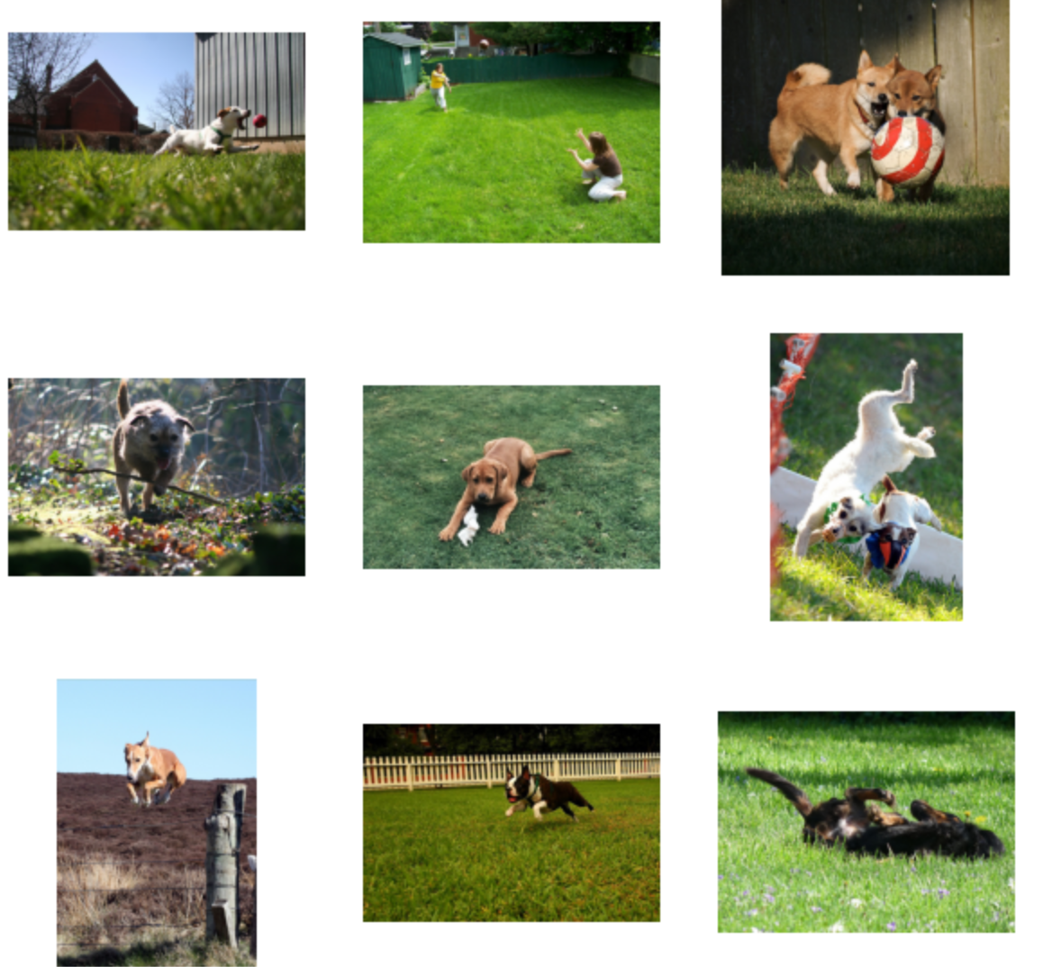
Some example(9 pic for every sentences):
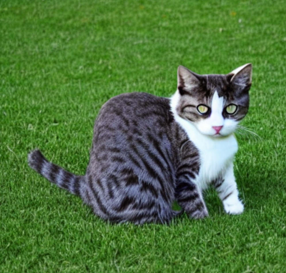
The image shows cats on the grass. The image shows dogs on the grass.
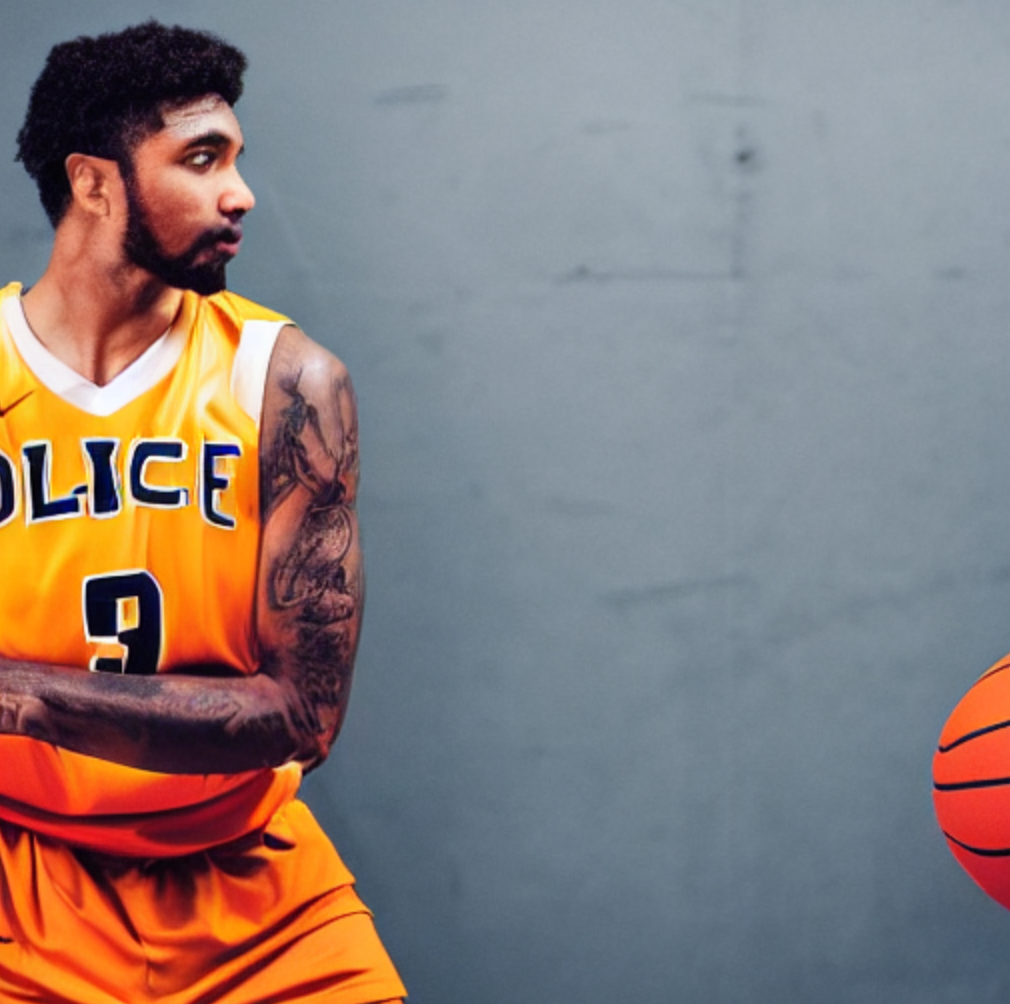
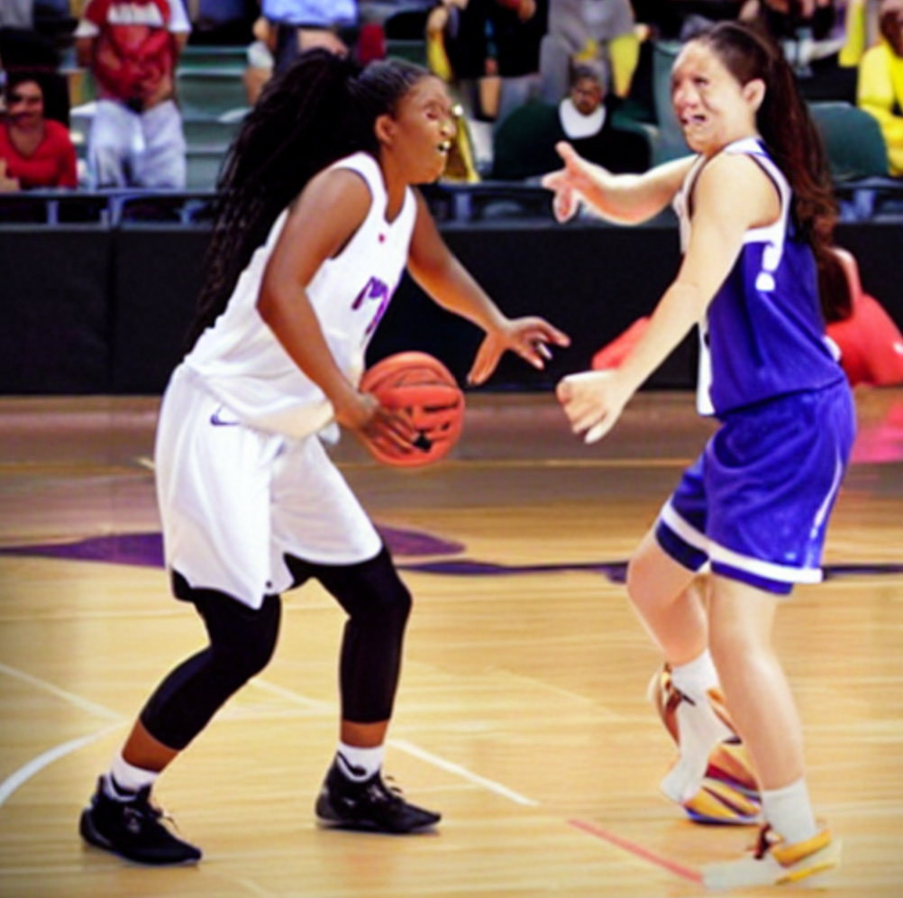
The image shows a man plays basketball. The image shows a women plays basketball.
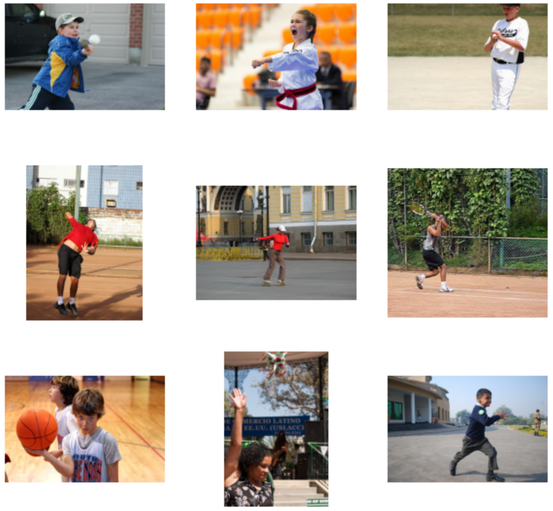
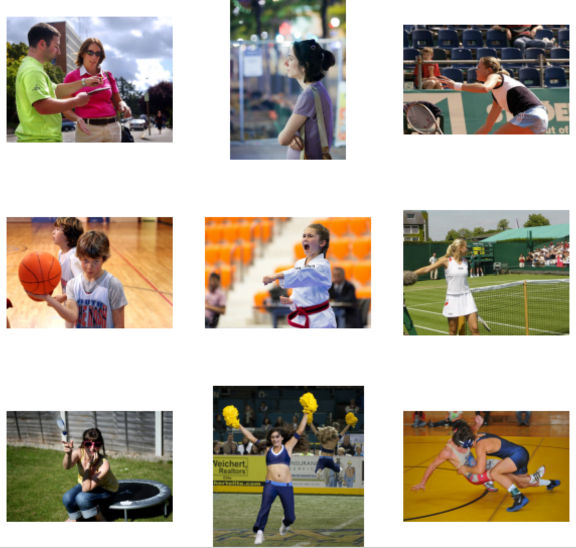
In these images, it can be seen that the model has indeed learned some features that correspond to text and images. For example, in this image, the grass, man, woman, plays, basketball can be recognized, but it can also be seen that the model has not understood some image features, such as the cat, nor the meaning of the relative relationship between sentences.
Review
I use the simple CLIP encoder can match images and text inputs that describe the same visual content. For example, given an image of a dog and a text input that says “dogs in the grass”, the CLIP encoder can recognize that the text input describes the image and assign a high similarity score to the pair.
What else can CLIP model do?
Applications
GLIDE:
The GLIDE[5] paper explores two different techniques for guiding diffusion models in text-conditional image synthesis. Classifier-free guidance replaces the label in a class-conditional diffusion model with a null label with a fixed probability during training. During sampling, the output of the model is extrapolated further in the direction of the label and away from the null label. Classifier-free guidance has two appealing properties: it allows a single model to leverage its own knowledge during guidance, and it simplifies guidance when conditioning on information that is difficult to predict with a classifier. CLIP guidance involves using a CLIP model, which is a scalable approach for learning joint representations between text and images, to replace the classifier in classifier guidance. The reverse-process mean is then perturbed with the gradient of the dot product of the image and caption encodings with respect to the image.
CLIP-NeRF:
In CLIP-NeRF paper[6], the authors propose a method for manipulating 3D objects using neural radiance fields (NeRF). The method uses a joint language-image embedding space of the CLIP model to allow for user-friendly manipulation of NeRF using either a short text prompt or an exemplar image. The authors introduce a disentangled conditional NeRF architecture that allows individual control over both shape and appearance. They also design two code mappers that take a CLIP embedding as input and update the latent codes to reflect the targeted editing. The mappers are trained with a CLIP-based matching loss to ensure manipulation accuracy. Additionally, the authors propose an inverse optimization method that accurately projects an input image to the latent codes for manipulation to enable editing on real images. The method is evaluated through extensive experiments on a variety of text prompts and exemplar images, and an intuitive interface for interactive editing is provided.
Simple GLIDE Implement
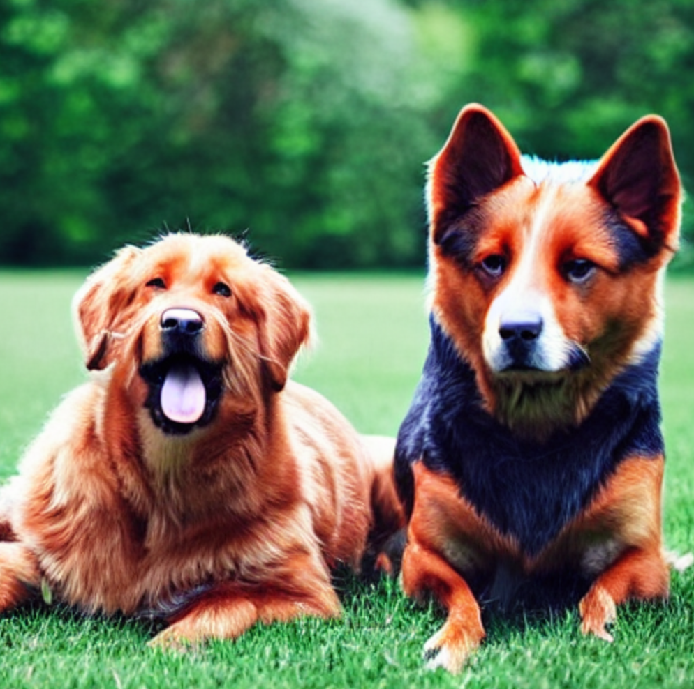
I show some results of the simple CLIP-guide diffusion model.
dogs on the grass. cats on the grass.
A man plays basketball. A women plays basketball.
Discussion
With the increasing number of recently released language models, it is foreseeable that CV models will also become larger and larger. For example, the CLIP model, as well as the EVA (1B) model distilled from the CLIP model. However, in this current “large model competition,” more and more resources are required, such as more training time and more GPUs. What can people with limited resources do in this kind of “large model competition”?
Maybe there is an example of one answer: This is a video model based on the CLIP approach[6]. The idea presented in this article is very appealing. In addition to fine-tuning some pre-trained models, we could also try adding adapters to the original model parameters freezing the original model parameters, just like adding FC layers to the original model as we learned in class. Perhaps this method will give us better results with limited computing resources.
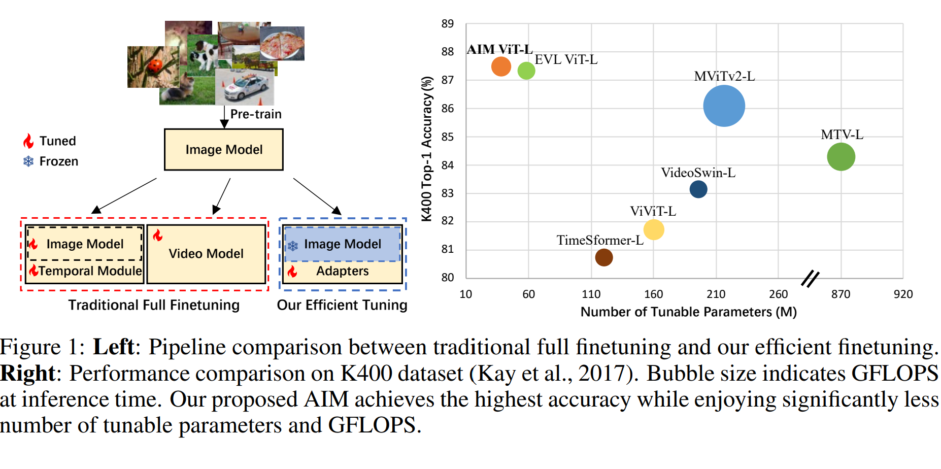
Fig 6. AIM: ADAPTING IMAGE MODELS FOR EFFICIENT VIDEO ACTION RECOGNITION [7].
You can refer to the source code for article structure ideas or Markdown syntax. We’ve provided a sample post and you can find the source code here
Reference
[1] Radford, Alec et al. “Learning Transferable Visual Models From Natural Language Supervision.” International Conference on Machine Learning 2021.
[2] Chen et al. “A Simple Framework for Contrastive Learning of Visual Representations.” ICML 2020.
[3] He, Fan et al. “Momentum Contrast for Unsupervised Visual Representation Learning.” CVPR 2020.
[4] Li, Fan et al. “Scaling Language-Image Pre-training via Masking.” 2023 ICLR. arXiv:2212.00794.
[5] Nichol, Dhariwalet al. “GLIDE: Towards Photorealistic Image Generation and Editing with Text-Guided Diffusion Models.” arXiv:2112.10741.
[6] Wang, Chai et al. “CLIP-NeRF: Text-and-Image Driven Manipulation of Neural Radiance Fields.” CVPR(2022). arXiv:2112.05139.
[7] Yang, Zhu et al. “AIM: ADAPTING IMAGE MODELS FOR EFFICIENT VIDEO ACTION RECOGNITION.” 2023 ICLR.