Panoptic Scene Graph Generation and Panoptic Segmentation

In this post, we’ll explore what panoptic scene graph generation and panoptic segmentation are, their implementation, and potential applications.

Introduction
Problem Definition
Method and Implementation
Evaluation and Results
Discussion
Three Most Relevant Research Papers
References

Introduction

In this report, we will explore panoptic scene graph generation and panoptic segmentation and walk through the implementation of these two tasks using the OpenPSG repository. We’ll then evaluate the robustness of the model, discuss the results, and explore the potential for improvement through fine-tuning or transfer learning.

Problem Definition

In this section, we’ll define panoptic segmentation and panoptic scene graph generation, explain how they differ from each other, and how they differ from related tasks such as semantic segmentation, instance segmentation, and scene graph generation.

Things vs. Stuff

First, we need to understand the difference between things and stuff. Things are objects like people, animals, and items. Stuff are background elements like grass, the sky, and the road.

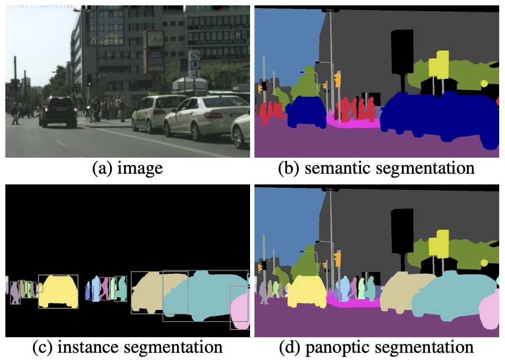
Semantic Segmentation

Semantic segmentation is the task of assigning a class label to each pixel in an image. These class labels can be either things or stuff. However, semantic segmentation doesn’t differentiate between different instances of the same class. For example, if there are two people in the image, they will get the same class label and are indistinguishable from each other on output.

Instance Segmentation

Instance segmentation is the task of detecting and segmenting each object instance in an image. These labels are only for things and doesn’t include stuff. For example, if there are two people in the image, they will get different class labels.

Panoptic Segmentation

Panoptic segmentation combines the semantic and instance segmentation tasks. It detects and segments different classes of objects as well as different instances of the same class. Each pixel is labeled with a class and instance ID. It also includes both things and stuff classes. For example, if there are two people in the image, they will get the same class label of “person” but different instance IDs to differentiate between them.

Scene Graph Generation

Scene graph generation takes an image and outputs a scene graph describing the objects and their relationships to each other. In a scene graph, each node represents an object and each edge represents a relationship between two objects. For example, if a person is holding a bag, the scene graph would have two nodes (person and bag) and one edge (person holding bag) connecting them. Regular scene graph generation doesn’t include stuff classes and uses bounding boxes.

Panoptic Scene Graph Generation

Panoptic scene graph generation is a combination of panoptic segmentation and scene graph generation. It also takes an image and outputs a scene graph describing the objects and their relationships to each other, but it also includes stuff classes and uses segmentation masks instead of bounding boxes. This allows it to give a more comprehensive description of the scene.

Comparison of Tasks

Comparison of instance, semantic, panoptic segmentation

Task	Things vs. Stuff	Instance Differentiation	Relationships	Output Format
Semantic Segmentation	Both	No	No	Segmentation masks
Instance Segmentation	Things only	Yes	No	Segmentation masks
Panoptic Segmentation	Both	Yes	No	Segmentation masks
Scene Graph Generation	Things only	Yes	Yes	Graph
Panoptic Scene Graph Generation	Both	Yes	Yes	Graph & Segmentation masks

Method and Implementation

To explore panoptic scene graph generation, we’ll use the OpenPSG repository. This repo contains the code, models, and data for the paper Panoptic Scene Graph Generation. First, we’ll discuss the OpenPSG models and then walk through the implementation.

OpenPSG

OpenPSG has various models they built and trained for panoptic scene graph generation, including both two-stage and one-stage models. The two-stage models first extract object features, masks, and class predictions using pretrained panoptic segmentation models of Panoptic FPN (Feature Pyramid Network). Then, they process these outputs using a relation prediction from scene graph generation methods such as IMP (Iterative Message Passing), MOTIFS, VCTree (Visual Concept Tree), and GPSNet (Graph Property Sensing Network). The one-stage models PSGTR and PSGFormer are based on DETR (Detection Transformer) (https://arxiv.org/abs/2005.12872), a transformer-based object detector. They predict triples (subject, predicate, object groups) and localizations (location of things and stuff) simultaneously.

Implementation

Environment Setup

Important note: If you want to run this code on Google Colab, you’ll need to downgrade CUDA to 10.1 with the following code in a notebook cell. If you’re running this locally, you may be able to skip this step depending on if you’re using CUDA and what version it is.

!wget https://developer.download.nvidia.com/compute/cuda/repos/ubuntu1810/x86_64/cuda-repo-ubuntu1810_10.1.105-1_amd64.deb
!yes | sudo dpkg -i cuda-repo-ubuntu1810_10.1.105-1_amd64.deb
!sudo apt-key adv --fetch-keys https://developer.download.nvidia.com/compute/cuda/repos/ubuntu1810/x86_64/7fa2af80.pub
!sudo apt-get update
!sudo DEBIAN_FRONTEND=noninteractive apt-get install cuda

First, install the required dependencies.

pip install torch torchvision torchaudio --index-url https://download.pytorch.org/whl/cu118
pip install openmim
mim install mmdet
mim install mmcv-full
pip install 'git+https://github.com/facebookresearch/detectron2.git'

pip install git+https://github.com/cocodataset/panopticapi.git
pip install xmltodict

Second, clone the OpenPSG repository.

git clone https://github.com/Jingkang50/OpenPSG.git

Next, download the checkpoint(s) you want to use. We’ll be using PSGTR and PSGFormer for this report. The checkpoint download links can be found in the OpenPSG README. I’ll be downloading it from Google Drive.

gdown 11zsy4yt9PFVXS-tJM8I5CiwYO5LposZC -O checkpoints/psgtr_r50.pth

Next, add the OpenPSG directory to your path.

import sys
sys.path.append('OpenPSG')

Finally, you can set all the seeds to make the results reproducible.

# code from https://gist.github.com/ihoromi4/b681a9088f348942b01711f251e5f964#file-seed_everything-py
def seed_everything(seed: int):
    import random, os
    import numpy as np
    import torch
    random.seed(seed)
    os.environ['PYTHONHASHSEED'] = str(seed)
    np.random.seed(seed)
    torch.manual_seed(seed)
    torch.cuda.manual_seed(seed)
    torch.backends.cudnn.deterministic = True
    torch.backends.cudnn.benchmark = True

seed_everything(42)

Testing the Model

Now that the environment is set up, we can initialize the model and run inference on custom images. All of this code is also used in the Colab demo and video demo.

import cv2
import mmcv
import torch
import urllib.request
import uuid
import numpy as np
import networkx as nx
import matplotlib.pyplot as plt
from mmcv import Config
from detectron2.utils.colormap import colormap
from detectron2.utils.visualizer import Visualizer
from mmdet.apis import init_detector, inference_detector
from mmdet.datasets.coco_panoptic import INSTANCE_OFFSET

CLASSES = [
    'person', 'bicycle', 'car', 'motorcycle', 'airplane', 'bus', 'train',
    'truck', 'boat', 'traffic light', 'fire hydrant', 'stop sign',
    'parking meter', 'bench', 'bird', 'cat', 'dog', 'horse', 'sheep', 'cow',
    'elephant', 'bear', 'zebra', 'giraffe', 'backpack', 'umbrella', 'handbag',
    'tie', 'suitcase', 'frisbee', 'skis', 'snowboard', 'sports ball', 'kite',
    'baseball bat', 'baseball glove', 'skateboard', 'surfboard',
    'tennis racket', 'bottle', 'wine glass', 'cup', 'fork', 'knife', 'spoon',
    'bowl', 'banana', 'apple', 'sandwich', 'orange', 'broccoli', 'carrot',
    'hot dog', 'pizza', 'donut', 'cake', 'chair', 'couch', 'potted plant',
    'bed', 'dining table', 'toilet', 'tv', 'laptop', 'mouse', 'remote',
    'keyboard', 'cell phone', 'microwave', 'oven', 'toaster', 'sink',
    'refrigerator', 'book', 'clock', 'vase', 'scissors', 'teddy bear',
    'hair drier', 'toothbrush', 'banner', 'blanket', 'bridge', 'cardboard',
    'counter', 'curtain', 'door-stuff', 'floor-wood', 'flower', 'fruit',
    'gravel', 'house', 'light', 'mirror-stuff', 'net', 'pillow', 'platform',
    'playingfield', 'railroad', 'river', 'road', 'roof', 'sand', 'sea',
    'shelf', 'snow', 'stairs', 'tent', 'towel', 'wall-brick', 'wall-stone',
    'wall-tile', 'wall-wood', 'water-other', 'window-blind', 'window-other',
    'tree-merged', 'fence-merged', 'ceiling-merged', 'sky-other-merged',
    'cabinet-merged', 'table-merged', 'floor-other-merged', 'pavement-merged',
    'mountain-merged', 'grass-merged', 'dirt-merged', 'paper-merged',
    'food-other-merged', 'building-other-merged', 'rock-merged',
    'wall-other-merged', 'rug-merged', 'background'
]

PREDICATES = [
    'over', 'in front of', 'beside', 'on', 'in', 'attached to', 'hanging from',
    'on back of', 'falling off', 'going down', 'painted on', 'walking on',
    'running on', 'crossing', 'standing on', 'lying on', 'sitting on',
    'flying over', 'jumping over', 'jumping from', 'wearing', 'holding',
    'carrying', 'looking at', 'guiding', 'kissing', 'eating', 'drinking',
    'feeding', 'biting', 'catching', 'picking', 'playing with', 'chasing',
    'climbing', 'cleaning', 'playing', 'touching', 'pushing', 'pulling',
    'opening', 'cooking', 'talking to', 'throwing', 'slicing', 'driving',
    'riding', 'parked on', 'driving on', 'about to hit', 'kicking', 'swinging',
    'entering', 'exiting', 'enclosing', 'leaning on',
]

def get_colormap(num_colors):
    return (np.resize(colormap(), (num_colors, 3))).tolist()

def draw_scene_graph(relations, rel_obj_labels):
    G = nx.DiGraph()

    # Add edges to the graph
    for subject_idx, object_idx, rel_id in relations:
        rel_label = PREDICATES[rel_id]
        G.add_edge(subject_idx, object_idx, label=rel_label)

    # Add nodes with connections to the graph
    connected_nodes = set()
    for u, v in G.edges():
        connected_nodes.add(u)
        connected_nodes.add(v)

    for node in connected_nodes:
        G.nodes[node]["label"] = rel_obj_labels[node]

    # Draw the graph
    plt.figure(figsize=(5, 5))

    # Customize graph
    pos = nx.kamada_kawai_layout(G)
    nx.draw(G, pos, node_size=1000, node_color="skyblue", with_labels=False)
    nx.draw_networkx_labels(G, pos, labels={node: G.nodes[node]["label"] for node in G.nodes()}, font_size=9, font_color="black")

    edge_labels = {(u, v): G.edges[u, v]["label"] for u, v in G.edges()}
    nx.draw_networkx_edge_labels(G, pos, edge_labels=edge_labels, font_size=9, font_color="red")

    plt.axis("off")
    plt.show()


def show_result(img, result, num_rel=20, title=None):
    img = img.copy()
    height, width = img.shape[:-1]

    # get panoptic results
    pan_results = result.pan_results
    ids = np.unique(pan_results)[::-1] # gets unique ids in reverse order
    num_classes = 133
    legal_idx = (ids != num_classes) # creates boolean array where elements are True if not num_classes, else False
    ids = ids[legal_idx]

    labels = np.array([id % INSTANCE_OFFSET for id in ids], dtype=np.int64)
    labels = [CLASSES[l] for l in labels]

    rel_obj_labels = result.labels
    rel_obj_labels = [CLASSES[l - 1] for l in rel_obj_labels]

    segments = pan_results[None] == ids[:, None, None]
    segments = [mmcv.image.imresize(segment.astype(float), (width, height)) for segment in segments]

    masks = result.masks

    colormap = get_colormap(len(masks))
    colormap = (np.array(colormap) / 255).tolist()

    # Visualize masks
    v = Visualizer(img)
    v.overlay_instances(
        labels=rel_obj_labels,
        masks=masks,
        assigned_colors=colormap
    )
    v_img = v.get_output().get_image()
    # print image to output
    plt.figure(figsize=(10, 10))
    if title is not None:
        plt.title(title)
    plt.imshow(v_img)
    plt.axis('off')
    # save image to file in directory `out` with a random name
    plt.savefig('out/' + str(uuid.uuid4()) + '.png', bbox_inches='tight', pad_inches=0, transparent=True)
    plt.show()

    # get relation results
    n_rel_topk = min(num_rel, len(result.labels) // 2)
    rel_dists = result.rel_dists[:, 1:] # Exclude background class
    rel_scores = rel_dists.max(1)
    rel_topk_idx = np.argpartition(rel_scores, -n_rel_topk)[-n_rel_topk:]
    rel_labels_topk = rel_dists[rel_topk_idx].argmax(1)
    rel_pair_idxes_topk = result.rel_pair_idxes[rel_topk_idx]

    relations = np.concatenate([rel_pair_idxes_topk, rel_labels_topk[..., None]], axis=1)

    draw_scene_graph(relations, rel_obj_labels)

    all_rel_visualizers = []

    for i, relation in enumerate(relations):
        subject_idx, object_idx, rel_id = relation
        subject_label = rel_obj_labels[subject_idx]
        object_label = rel_obj_labels[object_idx]
        rel_label = PREDICATES[rel_id]

        print(f"{subject_label} {rel_label} {object_label}")

        v = Visualizer(img)

        v.overlay_instances(
            labels=[subject_label, object_label],
            masks=[masks[subject_idx], masks[object_idx]],
            assigned_colors=[colormap[subject_idx], colormap[object_idx]],
        )

        v_masked_img = v.get_output().get_image()
        all_rel_visualizers.append(v_masked_img)

    return all_rel_visualizers

class Model:
    def __init__(self, ckpt, cfg, device="cpu"):
        config = Config.fromfile(cfg)
        self.device = device
        self.model = init_detector(config, ckpt, device=device)

    def predict(self, img_path, num_rel=20):
        img = cv2.imread(img_path)
        result = inference_detector(self.model, img_path)
        rel_images = show_result(img, result, num_rel=num_rel)
        return rel_images

def image_test(model, image_path, num_rel=20):
    if image_path.startswith("http"):
        image_filepath = "input_image.jpg"
        urllib.request.urlretrieve(image_path, image_filepath)
    else:
      image_filepath = image_path

    rel_images = model.predict(image_filepath, num_rel)

Now we can create a model by supplying the proper checkpoint and config file paths and test it on an image. image_test will output a visualization of the original image with masks overlaid for the detected objects (both things and stuff). It will also output the relations between objects in both a textual and graph format.

To test models besides PSGTR, we need to create config files dictating the inference pipeline since OpenPSG only provides an inference config for PSGTR. For example, to test PSGFormer, we can use the following config file (which is almost an exact copy of the PSGTR inference config OpenPSG/configs/psgtr/psgtr_r50_psg_inference.py) and place it in the OpenPSG/configs/psgformer directory:

_base_ = ["./psgformer_r50_psg.py"]

img_norm_cfg = dict(mean=[123.675, 116.28, 103.53], std=[58.395, 57.12, 57.375], to_rgb=True)
pipeline = [
    dict(type="LoadImageFromFile"),
    dict(
        type="MultiScaleFlipAug",
        img_scale=(1333, 800),
        flip=False,
        transforms=[
            dict(type="Resize", keep_ratio=True),
            dict(type="RandomFlip"),
            dict(type="Normalize", **img_norm_cfg),
            dict(type="Pad", size_divisor=32),
            # NOTE: Do not change the img to DC.
            dict(type="ImageToTensor", keys=["img"]),
            dict(type="Collect", keys=["img"]),
        ],
    ),
]

data = dict(
    test=dict(
        pipeline=pipeline,
    ),
)

model = Model("checkpoints/psgtr_r50.pth", "OpenPSG/configs/psgtr/psgtr_r50_psg_inference.py", device="cpu")
image_test(model, "input_image.jpg")

Example output:

Example output image

Example output graph

sky-other-merged over pavement-merged
person walking on road
person walking on pavement-merged
person riding bicycle
road attached to pavement-merged
person walking on pavement-merged
person walking on pavement-merged
person walking on pavement-merged
sky-other-merged over road
bicycle driving on road
person riding bicycle
person riding bicycle
sky-other-merged over building-other-merged

Demo

Google Colab Demo

Demo video

Video link

Evaluation and Results

To evaluate the performance of the OpenPSG PSGTR and PSGFormer models, I tested them on a diverse set of image inputs, including naturally-occurring adversarial images, images with occlusions, images with added noise, and images from real life.

Robustness Testing

Adversarial Images

When the model is tested on naturally-occurring adversarial images, or images that are not modified but are difficult for object recognition models to classify, it performs well for objects in its training data. It is able to recognize these objects and their relationships. However, for objects it hadn’t been trained on and didn’t have a class label for, it either classified them as the closest label or a completely unrelated label. This suggests that the model could potentially be improved by further training it on a more diverse dataset with more comprehensive class labels.

Occlusions

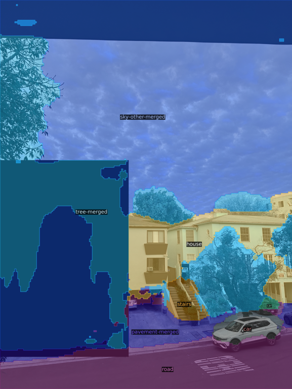
When tested on images with occlusions, the model performed very well and was able to recognize objects and their relations properly, even in cases where the occlusions span across multiple objects. This shows that the model is robust against partially visible objects, which is incredibly important for real-world applications. To further improve the model’s performance on occluded images, we could potentially use multiple views of the same scene to help the model better recognize these occluded objects.

Baseline image:

original image masked image

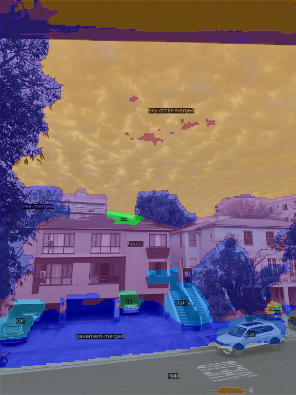
house beside tree-merged
car on road
sky-other-merged over road
sky-other-merged over house
car parked on road
car parked on road
sky-other-merged over tree-merged

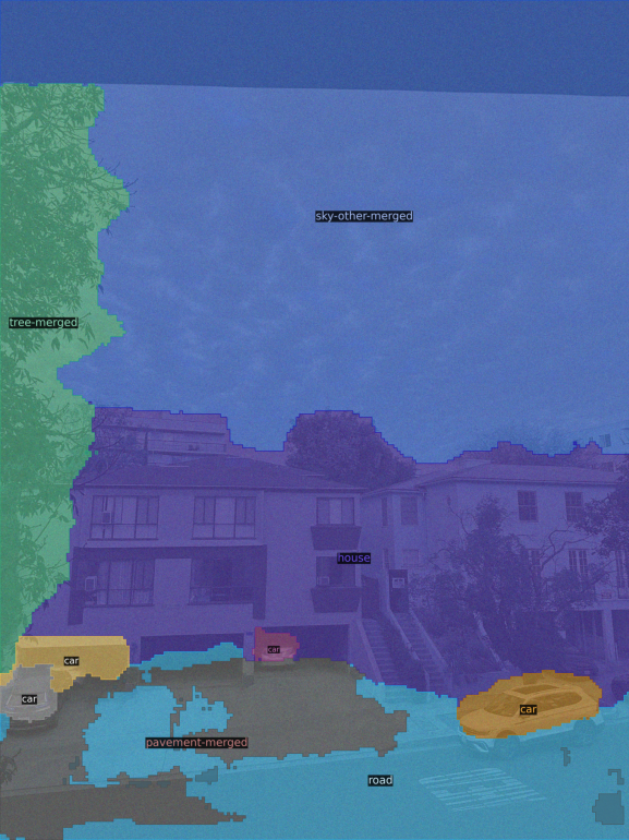
Example occluded image:

original image occluded image

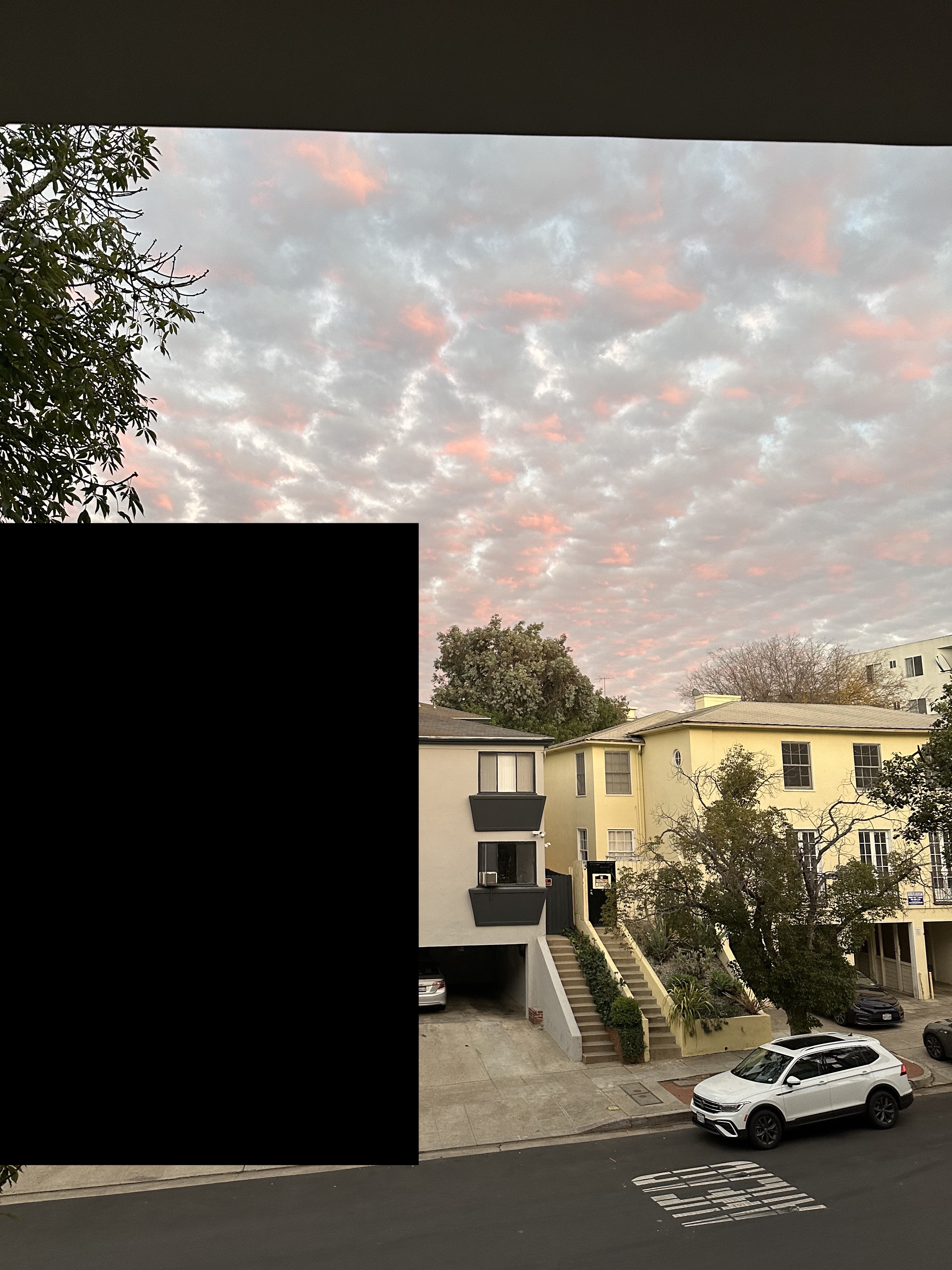
car parked on road
car parked on road
tree-merged beside house
sky-other-merged over tree-merged

Noise

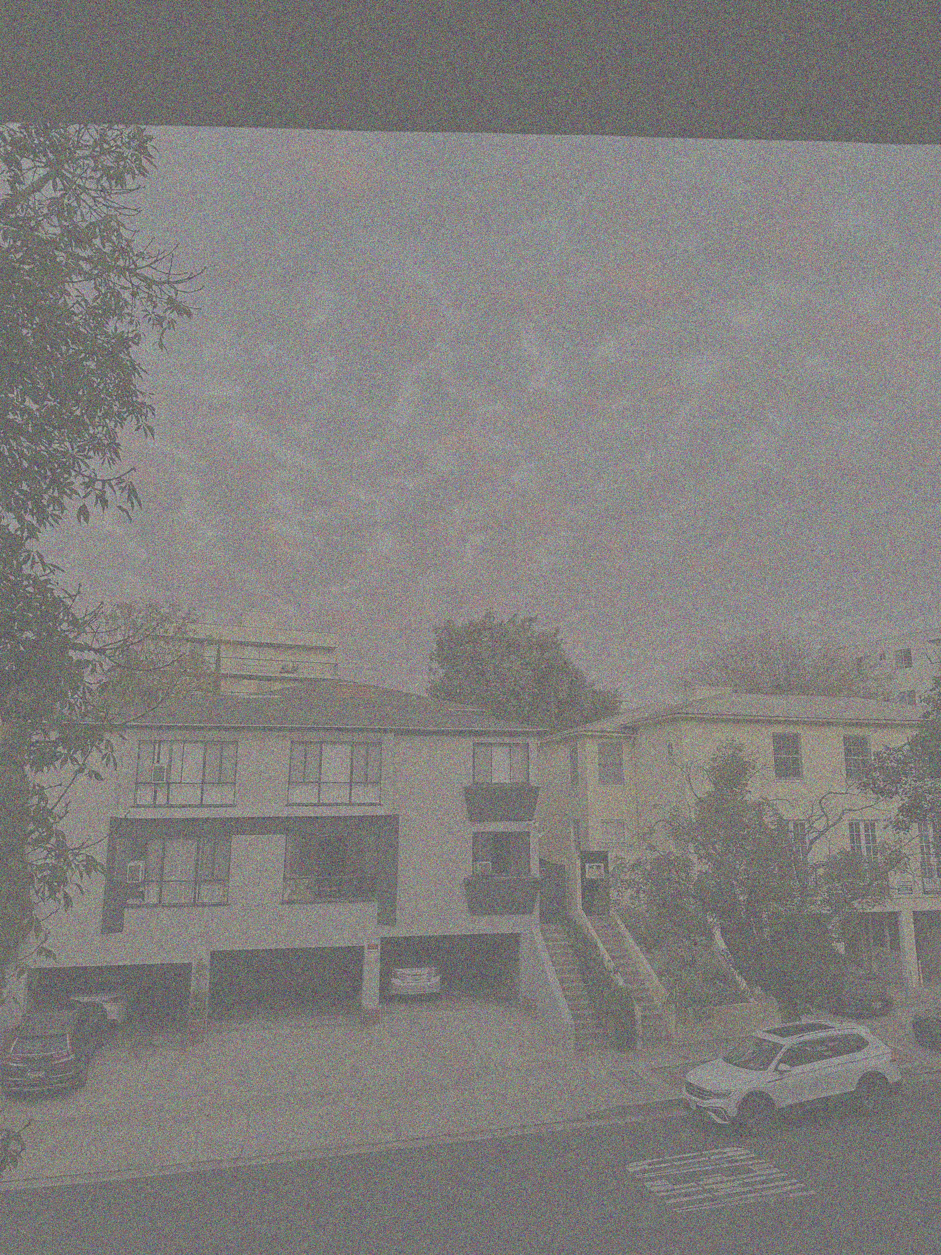
When tested on images with varying levels of noise added to them, the model performed very well and was able to recognize objects and their relationships, even up to 70% noise. Once the ratio reached 80% on real-life images, however, the model performed poorly and was unable to properly recognize objects. This shows ups that the model is very robust against noise, which is important for real-world applications since images are often noisy or have poor lighting. If we wanted to further improve the performance, we could use techniques such as denoising.

Example image with 70% noise:

original image noisy image

car beside house
car parked on road
car parked on road
sky-other-merged over tree-merged

Example image with 80% noise:

original image noisy image

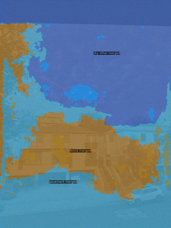
sky-other-merged beside pavement-merged

As we can see, the model loses most of its comprehension of the image at this point.

Real-life Images

When the model was tested on real-life images, it was very successful in recognizing objects and their relationships as long as the objects were in its training data and had a class label. In these cases, it provides a good amount of comprehension about the image, enough to potentially be useful for applications such as helping visually impaired users. Otherwise, it assigns the closest label. For example, it falsely assigns a fox as a dog or a cat. Through evaluation, I found that the biggest limitation of this model for real-life images is its training data and class labels.

Example image:

original image output image

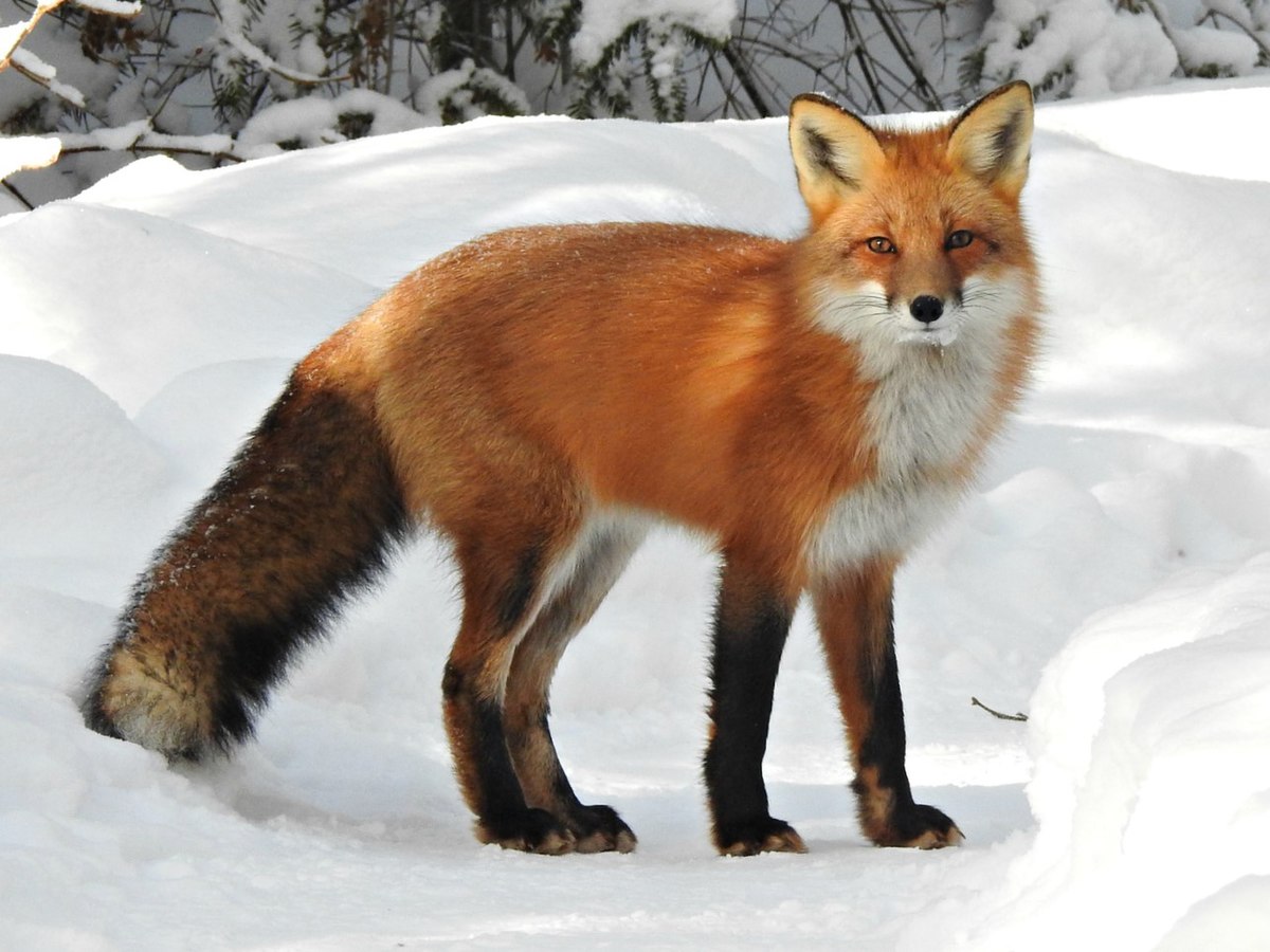
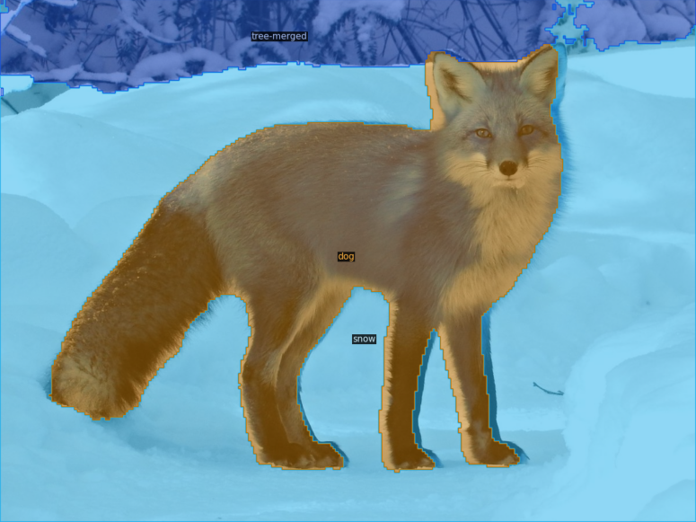
dog standing on snow

In summary, our comprehensive evaluation of the implemented OpenPSG model based on the PSGTR architecture showed promising results in terms of robustness and performance on real-life images. While there are some limitations, especially when dealing with unfamiliar objects, the model’s overall performance demonstrates its potential for practical applications and further improvement. By incorporating additional techniques and expanding the training dataset, the model can be refined to better handle challenging scenarios and provide more accurate scene graph generation in real-world situations.

Discussion

Fine-tuning and Transfer Learning

OpenPSG can be improved by using fine-tuning or transfer learning. In this section, I’ll discuss the potential benefits of these techniques.

Fine-tuning is when we take a pre-trained model train it on new data to improve its performance in that area. In this case, we could fine-tune the OpenPSG models on a more diverse dataset based on where its current weaknesses are. This will help the model better recognize these objects and their relationships. On the other hand, transfer learning is when we take a pre-trained model and use it on a new task/model. In this case, we could experiment with different backbone models to take advantage of their strengths.

Strengths and Weaknesses

As we discussed in the evaluation section, the OpenPSG models are robust to various types of adversarial images, such as occlusions and noise. They’re able to successfully recognize the objects and their relationships, keeping the majority of their comprehension about the image. However, they do have weaknesses, specifically when it comes to objects they hasn’t been trained on and don’t have class labels for. For example, it falsely assigns a fox as a dog or a cat as we saw above, and it fails to properly recognize a folded chair. To improve the performance of these models, we could train the model on a more diverse dataset with a wider range of class labels.

Three Most Relevant Research Papers

References

Kirillov, Alexander, et al. “Panoptic Segmentation.” ArXiv.org, 10 Apr. 2019, arxiv.org/abs/1801.00868.
Kirillov, Alexander, et al. “Panoptic Feature Pyramid Networks.” ArXiv.org, 8 Jan. 2019, arxiv.org/abs/1901.02446v2.
Yang, Jingkang, et al. “Panoptic Scene Graph Generation.” ArXiv.org, 22 July 2022, arxiv.org/abs/2207.11247.
Zhu, Guangming, et al. “Scene Graph Generation: A Comprehensive Survey.” ArXiv.org, 3 Jan. 2022, arxiv.org/abs/2201.00443.