Object Detection

In this project, we wish to dive deep and examine the YOLO v7 (You Only Look Once) object detection model while exploring any possible improvements. YOLO v7 is one of the fastest object detection models in the world today which provides highly accurate real-time object detection. During our examination, we will inspect the layers and algorithms within YOLO v7, test the pre-trained YOLO v7 model provided by the YOLO team, and train and test YOLO v7 against different datasets.

1. Introduction
2. Using and Training YOLOv7
- 2.1 Loading Pre-Trained Model
- 2.2 Training YOLOv7 On a Custom Dataset
3. Background of YOLO Models
4. YOLO v7
5. Potential Improvements
- 5.1 Anchor-Free Detection
- 5.2 Mosaic Augmentation
6. Conclusion
References and Code Bases

1. Introduction

The main idea behind the YOLO class of object detection algorithms is summarized in its acronym: “you only look once.” This means that YOLO models are single-stage, allowing them to immediately and accurately classify images. In fact, the speed is one of the major selling-points of this algorithm, allowing it to be marketed as a real-time object detector. It does this by immediately featurizing images before feeding the features into the model.

YOLO v7 is the latest in a line of YOLO object detection projects, beginning in 2015. Through each iteration, the YOLO models have become faster and more accurate by changing their base CNN structures, loss functions, and box-generation approaches.

The YOLO v7 model itself consists of three main parts, whith anatomical names to describe their functions: a backbone, neck, and head. The backbone is the first stage reached by the input. In it, the image is broken up into essential features. This feature data is then passed to the neck, in which feature pyramids are assembled, an extremely quick and high-quality, though expensive, method of feature extraction. The actual prediction part occurs in the head, which outputs detection boxes and prediction labels.

2. Using and Training YOLOv7

2.1 Loading Pre-Trained Model

Code Found In: Our Colab Notebook
Code Based Off: Official YOLOv7 Colab Notebook
Within the Official YOLOv7 repository, there are a few pre-trained YOLOv7 models that have been trained solely through the MS COCO Dataset. Some of these models are designed to work better on edge devices, such as YOLOv7-tiny, while others are designed to work better on stronger cloud devices, such as YOLOv7-W6. For the purposes of this demo, I will use the standard YOLOv7 pre-trained model.

Basic Setup: import sys, torch and clone the YOLOv7 repository.

import sys
import torch
!git clone https://github.com/WongKinYiu/yolov7

Download the pre-trained model:

!wget https://github.com/WongKinYiu/yolov7/releases/download/v0.1/yolov7.pt

Run object detection:

!python detect.py --weights yolov7.pt --conf 0.25 --img-size 640 --source inference/images/yolo-test1.jpg

Define helper function to view images and load image:

def imShow(path):
  import cv2
  import matplotlib.pyplot as plt
  %matplotlib inline

  image = cv2.imread(path)
  height, width = image.shape[:2]
  resized_image = cv2.resize(image,(3*width, 3*height), interpolation = cv2.INTER_CUBIC)

  fig = plt.gcf()
  fig.set_size_inches(18, 10)
  plt.axis("off")
  plt.imshow(cv2.cvtColor(resized_image, cv2.COLOR_BGR2RGB))
  plt.show()

imShow("runs/detect/exp5/yolo-test1.jpg")

detected image of friends on a hike

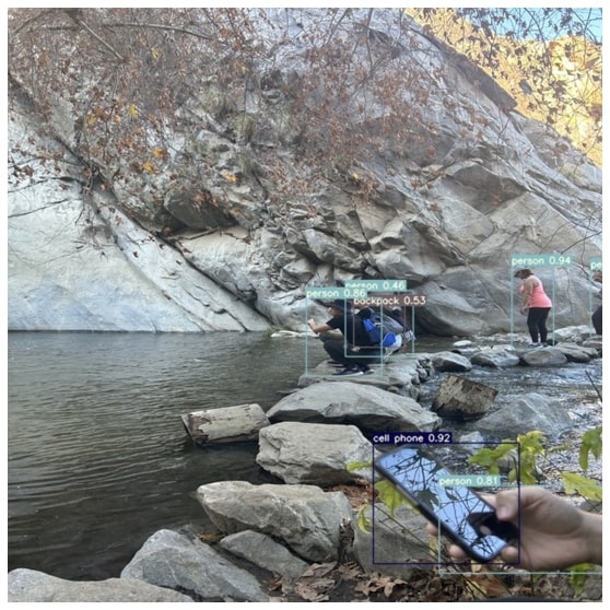
The pre-trained standard YOLOv7 model seems to work pretty well on a random image from my camera roll. It detects every person in the image as well as some objects with decent to good accuracy. Also, it completed object detection on this image on a T4 GPU in less than 5 seconds!

2.2 Training YOLOv7 On a Custom Dataset

The YOLOv7 models available online have all been trained exclusively with the MS COCO dataset. So although the pre-trained YOLOv7 model works well on regular object detection, we wanted to see if we could train our own dataset using YOLOv7 and test its efficacy.

2.2.1 Creating The Custom Dataset

The first step in training YOLOv7 on a custom dataset is creating the dataset. Since we aren’t curators of images, we decided to use images from Google Images. After installing the simple_image_download Python package, we wrote a simple script to download images from Google.

from simple_image_download import simple_image_download as simp

response = simp.simple_image_download

searches = ["bruin bear", "royce hall"]

for search in searches:
    response().download(search, 300)

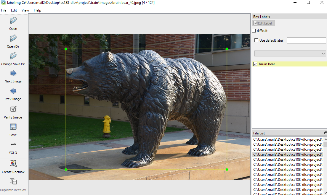
We downloaded 300 images of the bruin bear and 300 images of royce hall. Many of these images are not usable because they aren’t accurate visual representations of the desired objects, so we manually cut the images to around 70 of each category. After that, we used the labelImg Python library to create labels of each image. Using this package, we drew bounding boxes for each object within each image and the labels generated contain the coordinates for the bounding boxes, corresponding to each image.

labelImg bounding box drawing

We then created separate train and val folders with around 12 images and labels from each category in the validation folder and the remaining images and labels in the train folder. After that, we duplicated the standard YOLOv7.yaml cfg file and edited it to contain our custom class labels (‘bruin bear’ and ‘royce hall’) and train and val directory locations.

2.2.2 Training And Testing Custom Dataset

To train YOLOv7 on our custom dataset, we just had to run the following line of code:

!python train.py --device 0 --batch-size 16 --epochs 100 --img 640 640 --data data/custom_data.yaml --hyp data/hyp.scratch.custom.yaml --cfg cfg/training/yolov7-custom.yaml --weights yolov7.pt --name yolov7-custom

We decided to give ample time for training with 100 epochs and it took around 37 minutes to train. After training, all we had to do was use the best checkpoint from the model to detect our own images and videos. We took our own photos and videos of Royce Hall and the Bruin Bear to test this out. The line of code for running custom object detection is very similar to the one above which used the pre-trained model.

!python detect.py --weights runs/train/yolov7-custom/weights/best.pt --conf 0.5 --img-size 640 --source tests/royce_1.jpg --no-trace

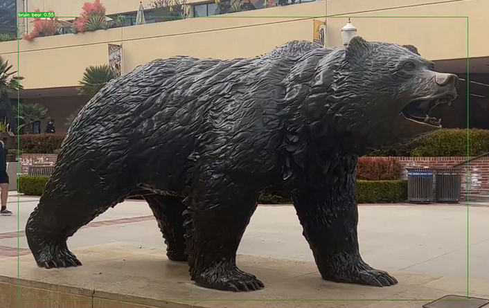
2.2.3 Results

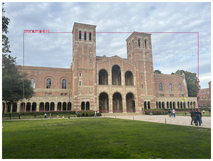
Here is an image of Royce Hall and a video of the Bruin Bear that we ran object detection on.

Royce Object Detection

click on the bruin bear image to watch the full video demo

YOLOv7 did pretty well on identifying Royce Hall, however, it did a little worse on identifying the Bruin Bear. In the full video of the bruin bear, it becomes more apparent that the model we trained does worse on the Bruin Bear. There are several factors which could have caused lower accuracy scores than we wanted such as the dataset being used was small, our bounding boxes weren’t drawn perfectly, our training hyperparameters weren’t ideal, and we didn’t use the other YOLOv7 models (such as YOLOv7x). But YOLOv7 is a one stage object detector, meant to detect objects fast, trading some accuracy along the way. And to that extent, it did a great job, taking only 0.8 seconds to run object detection on the Royce image and 14.8 seconds to run object detection on the 10 second long Bruin Bear video.

3. Background of YOLO Models

Object detection models in general can be classified into two main classes: two-stage (proposal) models, and one-stage (proposal-free) models. The two-stage models are mostly based on R-CNN (Region-based Convolutional Neural Network) structures. In this approach, the first step is to propose possible object regions. The second step is to compute features from these regions and formulate a conventional CNN to classify them. This approach is known to usually be very accurate; in fact, it generally is more accurate than one-stage models. Why do we sometimes use one-stage models then? To put it simply, they can be much faster, and in the object-detection world that is an enormous priority right now. One-stage models reject the region proposal step and proceed to run detection directly over a dense sampling of locations. A buzzword driving this push is “real-time” object detection, in which there is virtual no lag between images or video being observed and bounding boxes with classifications being returned. One such model is the one we are discussing here: YOLO. Only saying YOLO is perhaps a little too broad. Since its inception in 2016, the YOLO approach has been expanded upon by several different research groups into more than 7 different variations. Following the original YOLO paper, subsequent versions have added improvements to the head, neck, or backbone, and sometimes to multiple of these at a time. Below, we can see a summary of some of the architectural changes that took place during these evolutions.

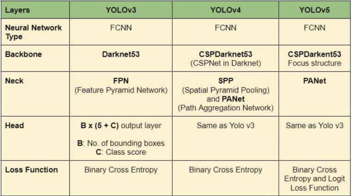
As we can see, these different YOLOs all use an FCNN, but their individual structures differ notably. To add to the confusion, not all advances in YOLO are sequential; in fact, YOLOv7 is based upon a version of YOLOv4 called Scaled YOLOv4 rather than YOLOv6 as we might expect. Despite this interrupted continuity, each version has improved in speed and accuracy.

4. YOLO v7

Hong-Yuan Mark Liao, the same group of researchers who developed scaled YOLOv4. One of the important distinguishing characteristics of this series of models is that they do not use pretrained ImageNet backbones, but are trained exclusively on the COCO (Common Objects in Context) dataset. As opposed to other large object detection datasets, COCO contains object segmentation information in addition to bounding box information, and each object is also annotated with textual captions (although they aren’t used in YOLO). But what does YOLO look like? Below is an excellent diagram showing the stages the make it up, and some details about what its CNN looks like:

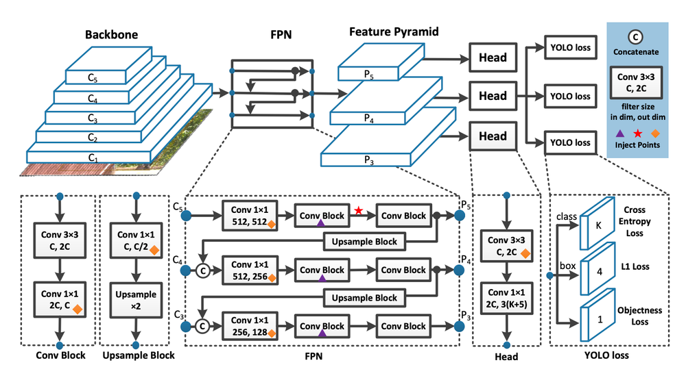
Though we will get into more detail below, we can define a useful summary of YOLO from the above: images are featurized in the backbone, these features are combined in the neck, and finally objects within the images are bounded and classified in the head. Our biggest focus here will be covering the advances made in YOLOv7 to improve on and differentiate from previous versions. Among these are the use of E-ELAN, Model Scaling techniques, and Planned Re-Parametrization.

4.1 Backbone

The first section of YOLOv7 is the backbone. As this model is one-stage rather than two-stage, it must immediately obtain features from its input without first running any predictions on the input data. The convolutional block that the authors settled on to make this happen is called E-ELAN (Exended Efficient Layer Aggregation). This is an improved version of regular ELAN. The ELAN architecture attempts to optimize network efficiency by controlling both shortest and longest gradient paths. The architecture itself looks relatively simple:

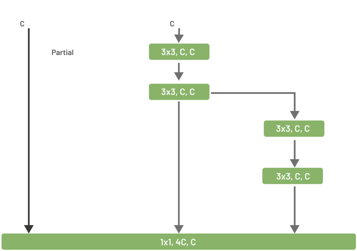
The bottom block is fed three different inputs. The first is just the original input, the second is passed through two blocks of 3 by 3 convolution, and the last is fed through to more of those blocks. In the bottom block, these 3 inputs are concatenated and put through a 1 by 1 convolution. E-ELAN is slightly more complex. It uses something called expand, shuffle, and merge cardinality to increase model learning while preserving the original path and allowing for continuous network learning improvement:

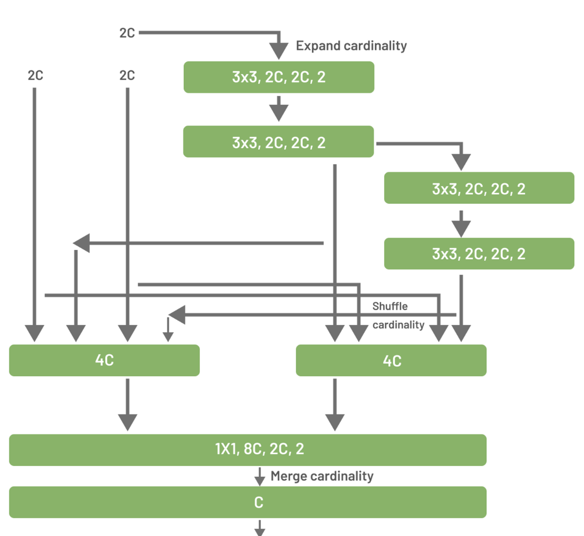
We can see that the pattern from the first illustration is maintained (direct input, input through two blocks, and input through four blocks), but the channels and cardinality of these blocks are expanded. Each computational block produces a feature map, which is shuffled and concatenated with the feature maps from the other blocks. At the end, this shuffled feature map from all the groups is added to get our final output. When this is done, our backbone has performed its requisite task, extracting features from out input. We now have our features and can proceed onto the neck.

4.2 Neck

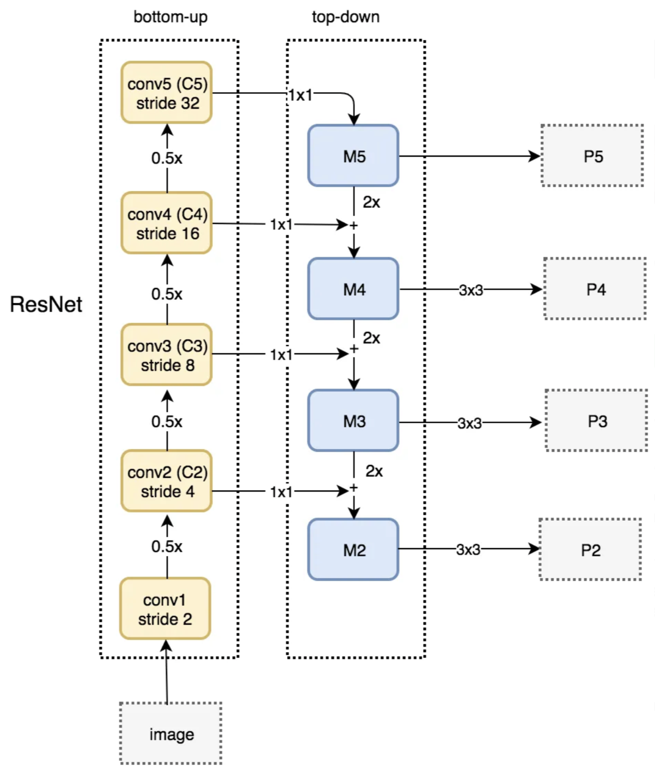
YOLOv7 uses a kind of bounding box called anchor boxes. This approach is important for our model because, unlike in two-stage model, we have not already made predictions for where objects must be, and are thus going into the bounding step blindly. In anchor boxing, a grid is drawn over the image and anchor points are generated at each grid intersection where a set of boxes of various sizes will be created. While this allows objects of almost any size in almost any image location to be bounded, it would be prohibitively expensive to cover every possible anchor box size. Thus, before anchor boxing occurs in the head, our neck must find a way to reduce the possible feature space of objects and thereby reduce the necessary number of anchor box sizes. To do this, YOLOv7 uses FPN (Feature Pyramid Networks). The goal of FPN is to quickly generate multiple layers of feature maps. To do this it uses a structure with two convolutional network pathways: bottom-up and top-down:

The bottom-up pathway is constructed using ResNet. It has five convolution modules, each with many layers. The stride is reduced by half at each sequential module, giving the output its pyramidal shape. The output of each convolutional module (C in the diagram) is also saved to be used in the second path (M in the diagram). After convolution module C5 is complete, the output is reduced in dimensionality by being passed through a 1x1 convolution and becomes M5, the first feature map layer. To get the next M layers, the output from the previous layer is upsampled by a factor of two and added with a 1x1 convolution of the corresponding C layer. Finally, that merged sum is put through a 3x3 convolution, yielding pyramid output feature map P. It is worth noting that only three or four such layers are used, with the bottom one or two being ignored due to the large dimensionality of C1 and C2. Were the last layers to be used, the process would become too slow for YOLOv7’s desired functionality.

4.3 Head

The head is where the actual predictions are made and the output labels and bounding boxes are returned. YOLOv7 improves upon previous versions by not only having one head. It uses something called auxiliary heads in addition to the lead head to make its classification. These auxiliary heads are updated as an intermediate layer to assist learning. During training, loss is calculated by assigning “soft labels” while training and comparing them to ground truth. The part that gives these labels is called the Label Assigner. A diagram of YOLOv7’s Coarse-to-fine lead guided assigner is below:

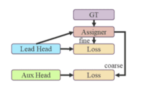
The final results on which soft labels are generated are predicted by the lead head, but both the lead head and auxiliary heads train on those predictions. In the YOLOv7 architecture there are actually two kinds of soft labels: course and fine, in which the coarse labels have higher sensitivity and therefore more possible error. The fine labels are used to train the lead head, while a set of coarse labels are used to train the auxiliary head. To boil the concept down a bit more, the main idea behind having these many heads is that the lead head can focus on learning the most important features while the auxiliary heads deal with the residual information.

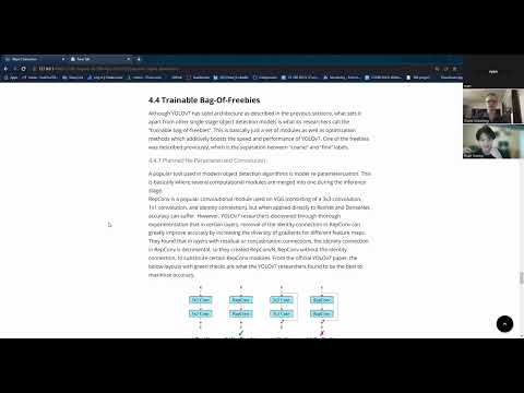
4.4 Trainable Bag-Of-Freebies

Although YOLOv7 has solid architecture as described in the previous sections, what sets it apart from other single-stage object detection models is what its researchers call the “trainable bag-of-freebies”. This is basically just a set of modules as well as optimization methods which additively boosts the speed and performance of YOLOv7. One of the freebies was described previously, which is the separation between “coarse” and “fine” labels.

4.4.1 Planned Re-Parameterized Convolution

A popular tool used in modern object detection algorithms is model re-parameterization. This is basically where several computational modules are merged into one during the inference stage.
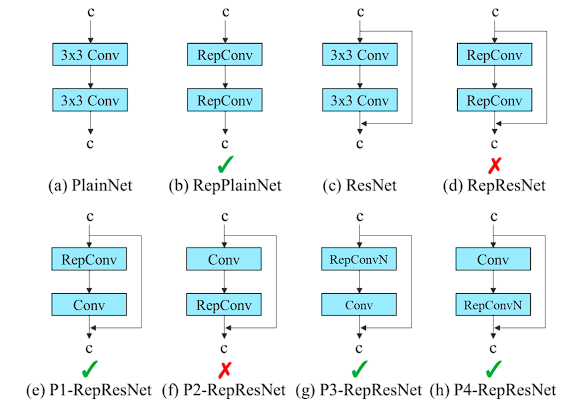
RepConv is a popular convolutional module used on VGG (consisting of a 3x3 convolution, 1x1 convolution, and identity connection), but when applied directly to ResNet and DenseNet, accuracy can suffer. However, YOLOv7 researchers discovered through thorough experimentation that in certain layers, removal of the identity connection in RepConv can greatly improve accuracy by increasing the diversity of gradients for different feature maps. They found that in layers with residual or concatenation connections, the identity connection in RepConv is detrimental, so they created RepConvN, RepConv without the identity connection, to substitute certain RepConv modules. From the official YOLOv7 paper, the below layouts with green checks are what the YOLOv7 researchers found to be the best to maximize accuracy.

4.4.2 Batch Normalization Attachment

YOLOv7 researchers also found that by attaching batch normalization directly to some convolutional layers, it can increase accuracy. They found that through integrating batch normalization’s mean and variance into a convolutional layer’s bias and weight during the inference stage, accuracy benefitted.

4.4.3 EMA Model

EMA stands for exponential moving average. YOLOv7 researchers use an EMA model to calculate an exponentially weighted moving average of model parameters which is maintained throughout the entire training run. This EMA is utilized during the inference stage, so instead of using the parameters from the last update, it uses this EMA. This is beneficial because it ‘smooths’ out the data. For example, if training was very poor during its early stages, the parameters could be drastically updated at the detriment of future batches. But by using EMA, any large updates would be smoothed out and have a less impactful effect on the parameters of the model.

5. Potential Improvements

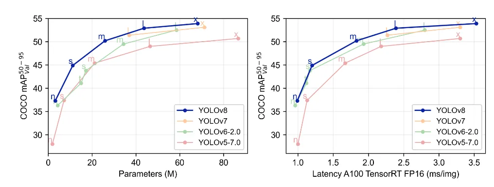
Although YOLOv7 is a state-of-the-art real-time object detection model, it was released in July 2022. Since then, researchers separate from YOLOv7 developed YOLOv8 which boasts better performance than YOLOv7 in both speed and accuracy. Below is an image from the YOLOv8 repository which shows YOLOv8 performing better than its predecessors on the COCO dataset.

5.1 Anchor-Free Detection

As shown previously, one of the main tools YOLOv7 utilizes is anchor boxes as their primary bounding boxes. However, YOLOv8 uses a completely anchor-free approach which directly predicts the center of an object instead of the offset from a known anchor box. This greatly reduces the number of box predictions that have to be made which speeds up the model.

5.2 Mosaic Augmentation

Another method that YOLOv8 utilizes which is not found in YOLOv7 is mosaic augmentation. Augmentation is where at each epoch, the model sees slightly altered versions of the images provided. Mosaic augmentation, used by YOLOv8, is where four images are stitched together and trained upon together instead of individually. This allows the model to learn objects that are found in new locations, potentially hidden, and against different surrounding pixels. This method has been found to decrease performance when trained through all epochs, so the YOLOv8 team specifically used it for certain training periods.

6. Conclusion

YOLOv7 is an incredibly fast and accurate real-time object detector which improves upon its previous iterations. The pre-trained YOLOv7 models are incredibly accessible and anyone could use them. Training YOLOv7 on custom data also proves to be effective, thus making it useful for real-world applications which require fast and accurate object detection. Although complex, YOLOv7’s architecture proves to stand strong against its competitors, however there are still many improvements to be made.