Image Generation

In the realm of image generation, deep learning technologies have revolutionized traditional methods, enabling advanced applications like text-to-image generation, style transfer, and image translation with unprecedented effectiveness. This blog highlights the transformative capabilities of deep learning for generating high-quality images. We will compare and contrast Generative Adversarial Networks (GANs) and diffusion models and show the strengths and applications of each model

Introduction
Fake Celebrity Image Generation with DCGAN
Monet Style Transfer with CycleGAN
Text-to-image Generation with Imagen
- Imagen Architecture
Implementation of MinImagen in PyTorch
Imagen Performance
- Quantitative performance
- Qualitative performance
Reference

Introduction

Image generation has emerged as one of the most fascinating and fast-developing areas in the field of computer vision and deep learning. With tasks ranging from creating fake images that are similar to inputs, to translating images to match a particular artistic style, the possibilities are expansive. These methods not only showcase the creative potential of AI but also highlight the intricate understanding these models have of content and style, foregrounding the nuanced interplay between them. This versatility and depth of understanding make deep learning an indispensable tool in the ongoing innovation within the realm of image generation.

Examples of AI Generated Images

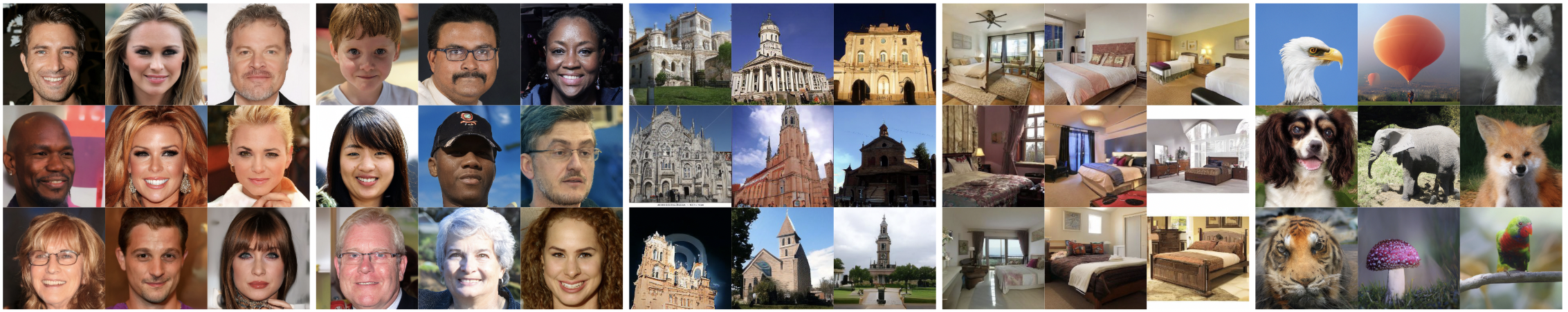
Fig 1. Examples of AI Generated Images (from Latent Diffusion Model) [1].

Specifically, we will discuss how deep learning is used for three image generation tasks:

1). Generating fake images that are similar to a set of inputs - The goal of generating images that are similar to a given input set is to produce new, unique images that maintain the essence of the original dataset. Deep learning models, particularly Generative Adversarial Networks (GANs), have shown exceptional prowess in this domain. They learn to replicate the complex distribution of the input images, enabling the generation of new images that, while novel, are visually indistinguishable from the originals.

Examples of face image generation

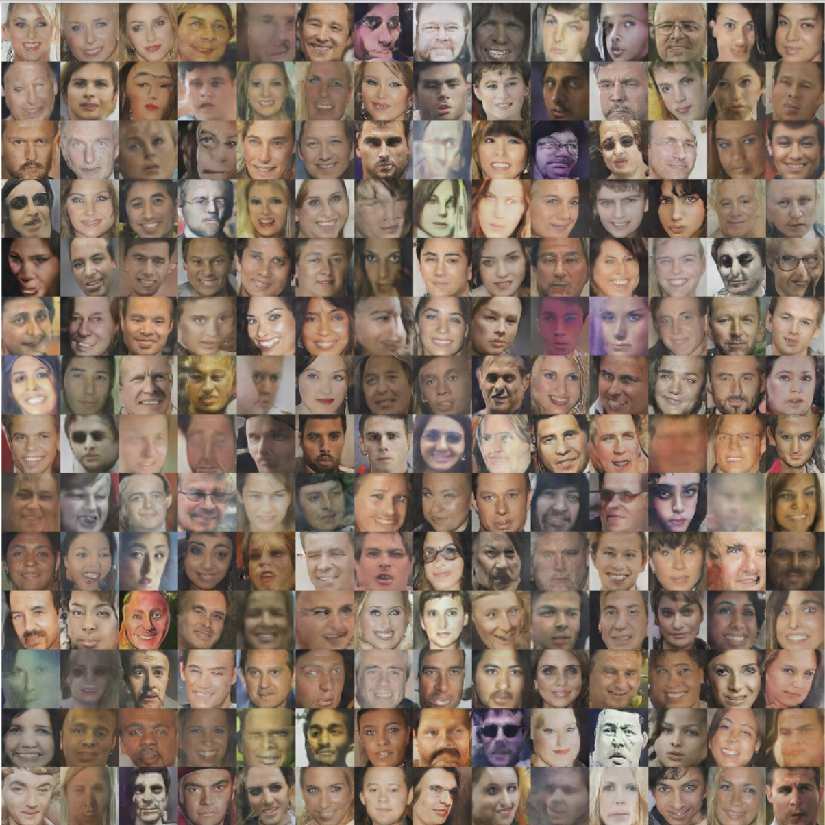
Fig 2. Examples of face images generated by Deep Convolutional GAN (DCGAN) [2].

2). Neural Style Transfer - Moving into the artistic domain, neural style transfer represents a particularly mesmerizing application of AI in image generation. Here, deep learning models—often a combination of Convolutional Neural Networks (CNNs) and GANs—are trained to dissect and understand the distinguishing features of an artist’s style and then apply it to any given photograph. The result is a harmonious blend that retains the structure of the original photo while adopting the artistic flair of the chosen style. This is not merely a pixel-level transformation but a deep structural reimagining of the image that reflects the unique artistic signatures of color, brushwork, and texture.

Examples of neural style transfer

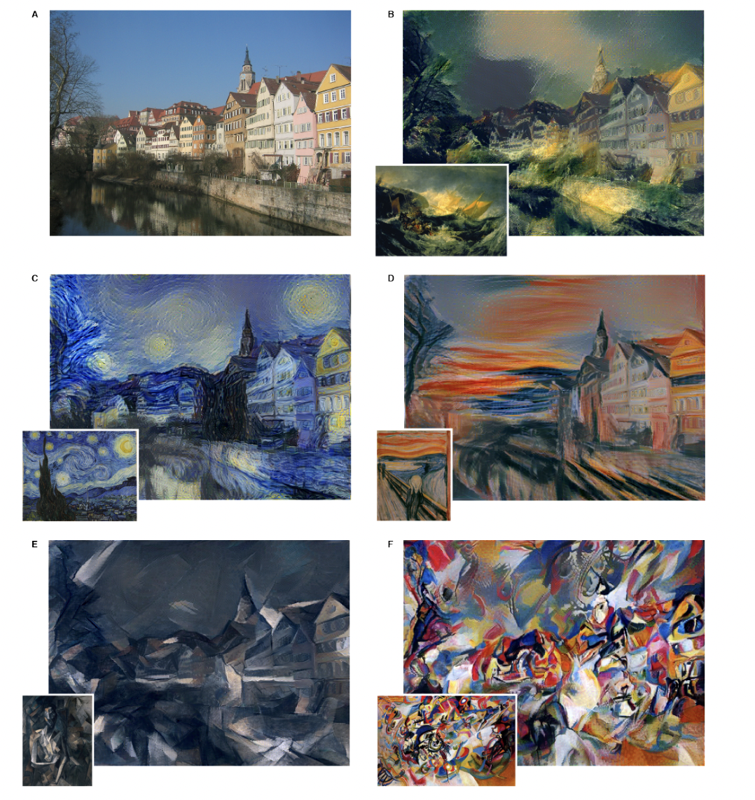
Fig 3. Examples of neural style transfer from CNN. Image A is input image and others are transformed copies of the input based on various art styles [3].

3). Text-to-image generation - Text-to-image generation stands out as a testament to the remarkable advancements in natural language processing and computer vision as models must be capable of both understanding the text inputs and generate a coherent image. . Models designed for this task take descriptive text as input and output images that accurately capture the described scenes or objects. Diffusion models work particularly well in this domain.

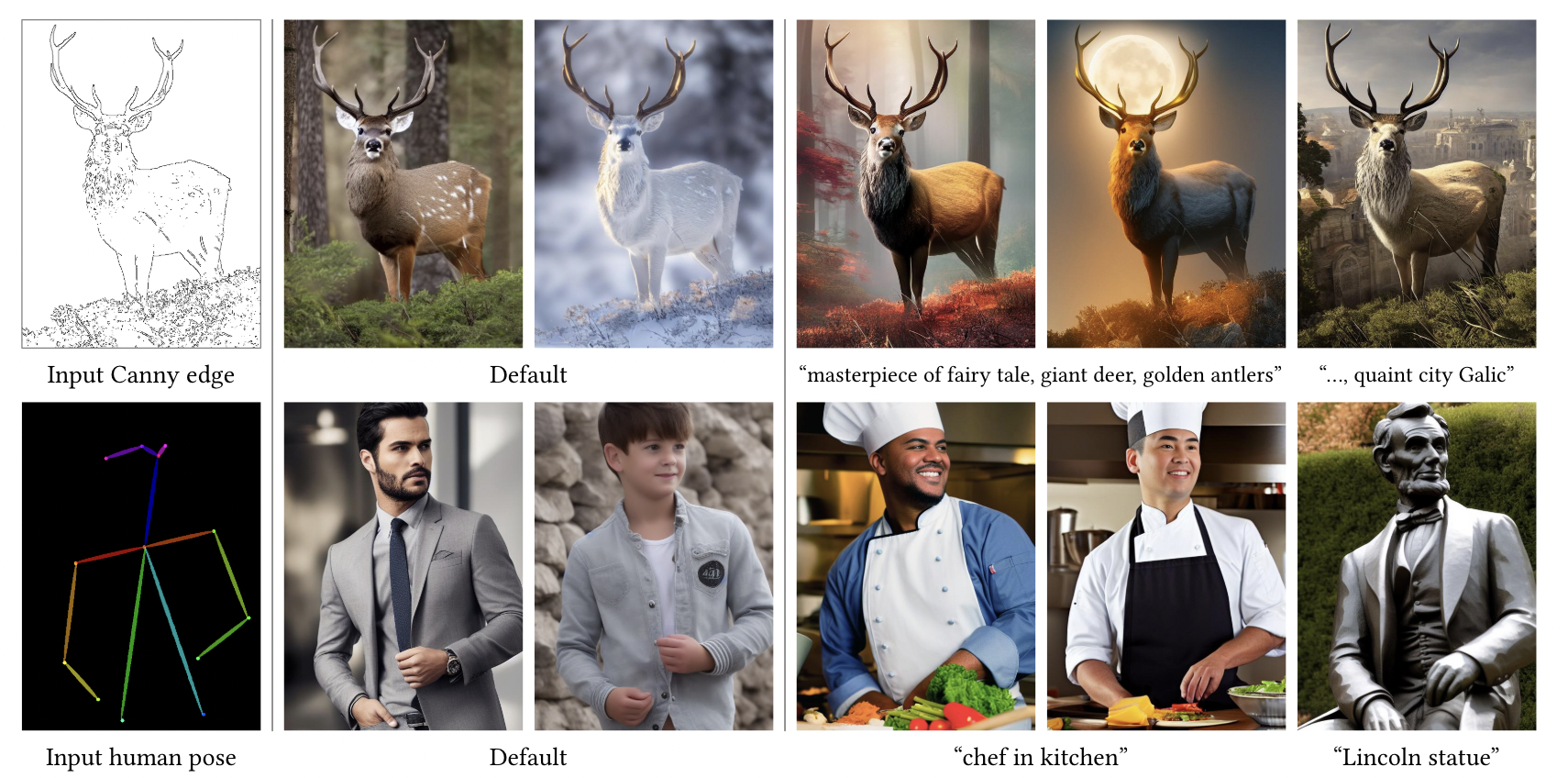
Examples of text-to-image generation

Fig 4. Examples of text-to-image generation from ControlNet [4].

In the remaining of this blog, we will discuss three deep learning models (one for each task) in detail and how they are able to accomplish the image generation tasks. Lastly, we will present the strength and weakness of each architecture and illustrate the potential trade-offs when choosing which architecture to use.

Fake Celebrity Image Generation with DCGAN

In this section, we will discuss Generative Adversarial Networks (GANs) and show how to create a Deep Convolutional GAN (DCGAN) to generate fake celebrity face images using the CelebA dataset.

GAN Architecture

GAN consists of two neural networks against each other in a game-theoretic scenario. The first network, known as the Generator, receives random input and is tasked with creating images that look as real as possible. The second network, called the Discriminator, evaluates an input image to determine whether it is real (from the dataset) or fake (produced by the Generator). Through iterative training, the Generator learns to produce increasingly realistic images, while the Discriminator becomes better at distinguishing real images from fakes.

GAN Architecture

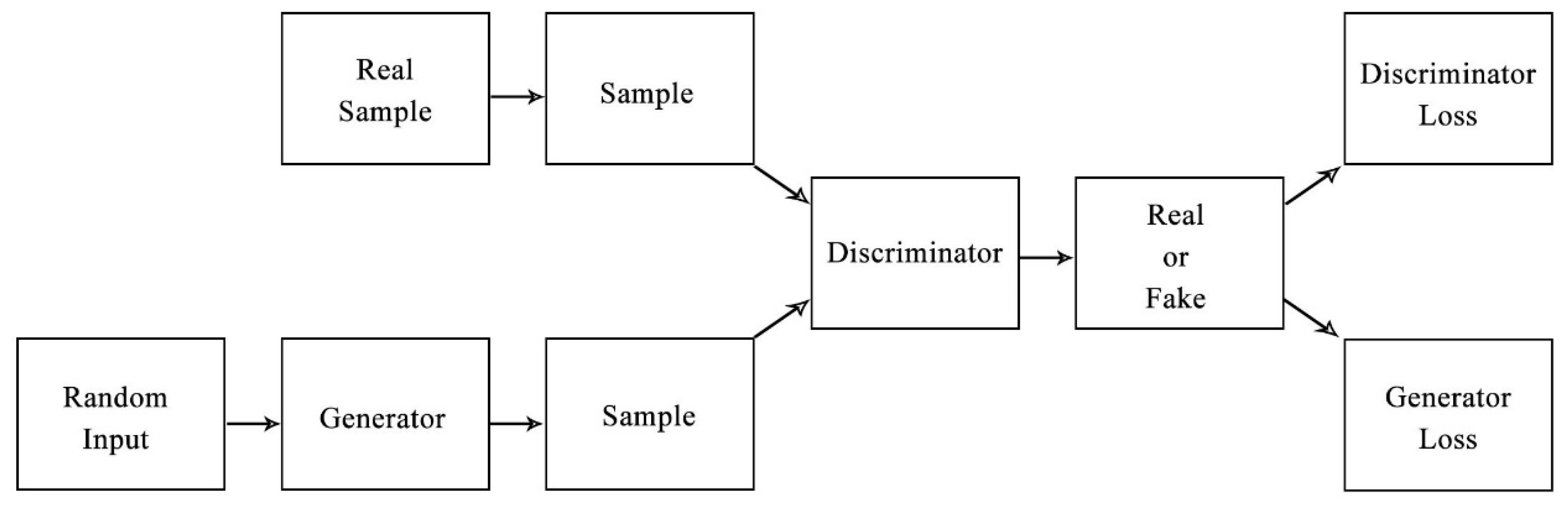
Fig 5. GAN Architecture [5].

Specifically, we define $x$ be an input image, $p_{\text{data}}$ be the probability $x$ is from image space, $D(x)$ be the discriminator output for $x$ (scalar probability that $x$ comes from dataset), $z$ be a latent space vector sampled from a standard normal distribution, $p_z(z)$ be the probability that $z$ is from latent vector space, and $G(z)$ be the generator output that maps $z$ to image space. $G$ wants to maximize the value of $D(G(z))$, which is the probability that the generator output is classified as comes from dataset (real), whereas $G$ wants to maximize $D(x)$, which is the probability that a real image is classified as real, and minimize $D(G(z))$. Hence, GAN loss function becomes:

\[\min_{G} \max_{D} V(D, G) = \mathbb{E}_{x \sim p_{\text{data}}(x)}[\log D(x)] + \mathbb{E}_{z \sim p_z(z)}[\log(1 - D(G(z)))]\]

The first term $\mathbb{E}_{x \sim p_{\text{data}}(x)}[\log D(x)]$ represents the expected log-probability of the discriminator being correct on real data, while the second term $\mathbb{E}_{z \sim p_z(z)}[\log(1 - D(G(z)))]$ represents the expected log-probability of the discriminator being correct on fake data generated by $G$.

DCGAN Architecture

DCGAN is an CNN-extension of GAN. DCGAN uses convolutional and convolutional-transpose layers in the discriminator and generator respectively. The generator architecture presented in DCGAN paper is shown below:

DCGAN Generator Architecture

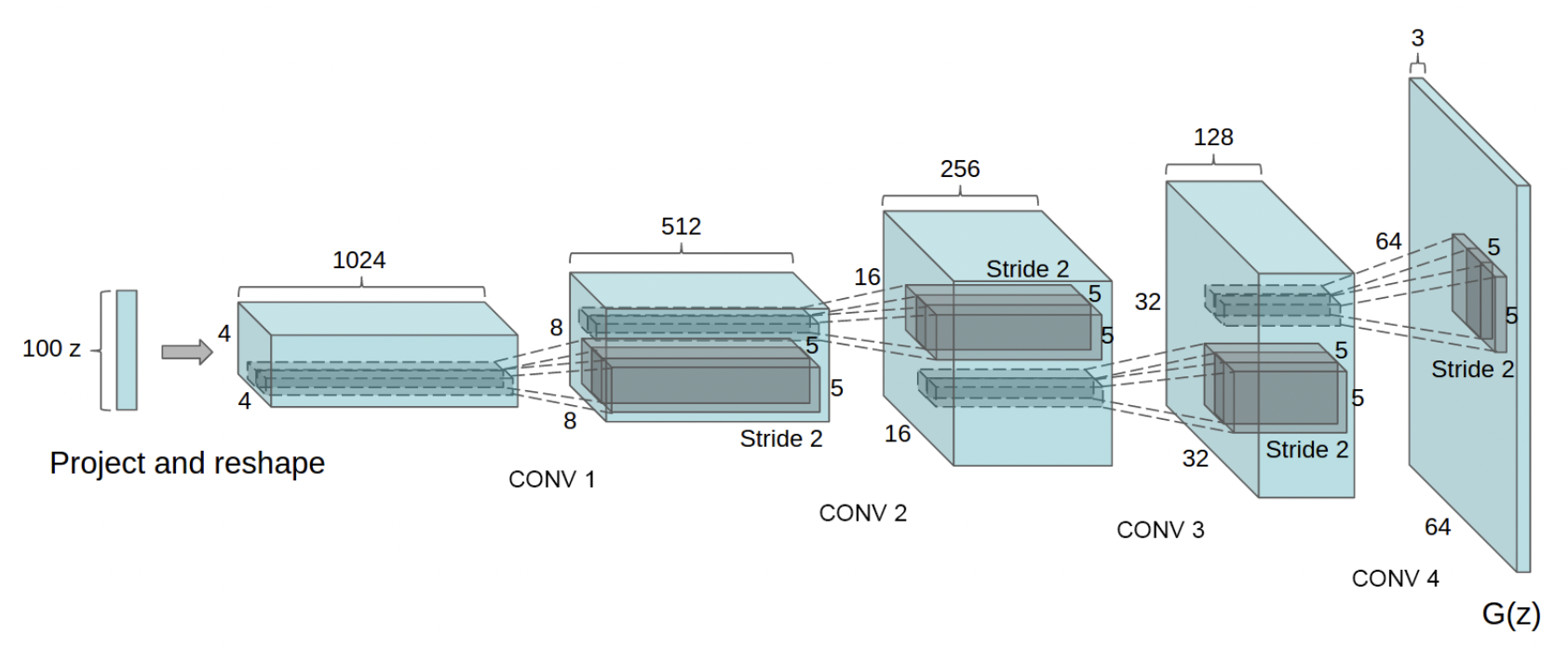
Fig 6. DCGAN Generator Architecture [2].

Implementation

Here, we will implement DCGAN and generate fake facial images using the CelebA dataset following Pytorch official tutorial. We will include some core code snippets for model architectures/weight initializations/etc. Fully implementation can be found in the tutorial.

First, let us visualize some example images from CelebA dataset:

CelebA Training Images

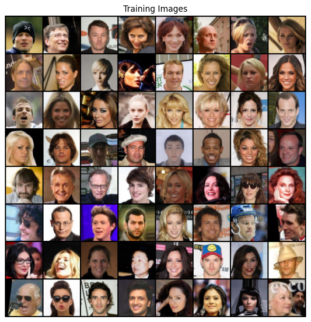
Fig 7. CelebA Training Images.

Weight Initialization

In the DCGAN paper, the author specified that all model weights should be randomly initialized from a normal distribution with mean = 0 and std = 0.2. We therefore define the weights_init method as follows:

# custom weights initialization called on netG and netD
def weights_init(m):
    classname = m.__class__.__name__
    if classname.find('Conv') != -1:
        nn.init.normal_(m.weight.data, 0.0, 0.02)
    elif classname.find('BatchNorm') != -1:
        nn.init.normal_(m.weight.data, 1.0, 0.02)
        nn.init.constant_(m.bias.data, 0)

Generator

As previously shown, the generator will map the latent space vector $z$ to image space. This is done through a series of transpoed 2d convolutions. Also, DCGAN innovatively adds batch norm layers after transposed convolutions, which help with the flow of gradients during training. Here nz is the length of the z input vector (in DCGAN case 100), ngf is the size of the feature maps that are propagated through the generator (in DCGAN case 64), and nc is the number of channels in the output image (set to 3 for RGB images)

# Generator Code

class Generator(nn.Module):
    def __init__(self, ngpu):
        super(Generator, self).__init__()
        self.ngpu = ngpu
        self.main = nn.Sequential(
            # input is Z, going into a convolution
            nn.ConvTranspose2d( nz, ngf * 8, 4, 1, 0, bias=False),
            nn.BatchNorm2d(ngf * 8),
            nn.ReLU(True),
            # state size. (ngf*8) x 4 x 4
            nn.ConvTranspose2d(ngf * 8, ngf * 4, 4, 2, 1, bias=False),
            nn.BatchNorm2d(ngf * 4),
            nn.ReLU(True),
            # state size. (ngf*4) x 8 x 8
            nn.ConvTranspose2d( ngf * 4, ngf * 2, 4, 2, 1, bias=False),
            nn.BatchNorm2d(ngf * 2),
            nn.ReLU(True),
            # state size. (ngf*2) x 16 x 16
            nn.ConvTranspose2d( ngf * 2, ngf, 4, 2, 1, bias=False),
            nn.BatchNorm2d(ngf),
            nn.ReLU(True),
            # state size. (ngf) x 32 x 32
            nn.ConvTranspose2d( ngf, nc, 4, 2, 1, bias=False),
            nn.Tanh()
            # state size. (nc) x 64 x 64
        )

    def forward(self, input):
        return self.main(input)

# Create the generator
netG = Generator(ngpu).to(device)

# Handle multi-gpu if desired
if (device.type == 'cuda') and (ngpu > 1):
    netG = nn.DataParallel(netG, list(range(ngpu)))

# Apply the weights_init function to randomly initialize all weights
#  to mean=0, stdev=0.2.
netG.apply(weights_init)

Discriminator

As mentioned, the discriminator is a binary classification network that takes an image as input and outputs a scalar probability that the input image is real (as opposed to fake). In our case, the discriminator takes in a 3 * 64 * 64 image. The DCGAN paper mentions it is a good practice to use strided convolution rather than pooling to downsample because it lets the network learn its own pooling function. Also batch norm and leaky relu functions promote healthy gradient flow which is critical for the learning process of both $G$ and $D$.

class Discriminator(nn.Module):
    def __init__(self, ngpu):
        super(Discriminator, self).__init__()
        self.ngpu = ngpu
        self.main = nn.Sequential(
            # input is (nc) x 64 x 64
            nn.Conv2d(nc, ndf, 4, 2, 1, bias=False),
            nn.LeakyReLU(0.2, inplace=True),
            # state size. (ndf) x 32 x 32
            nn.Conv2d(ndf, ndf * 2, 4, 2, 1, bias=False),
            nn.BatchNorm2d(ndf * 2),
            nn.LeakyReLU(0.2, inplace=True),
            # state size. (ndf*2) x 16 x 16
            nn.Conv2d(ndf * 2, ndf * 4, 4, 2, 1, bias=False),
            nn.BatchNorm2d(ndf * 4),
            nn.LeakyReLU(0.2, inplace=True),
            # state size. (ndf*4) x 8 x 8
            nn.Conv2d(ndf * 4, ndf * 8, 4, 2, 1, bias=False),
            nn.BatchNorm2d(ndf * 8),
            nn.LeakyReLU(0.2, inplace=True),
            # state size. (ndf*8) x 4 x 4
            nn.Conv2d(ndf * 8, 1, 4, 1, 0, bias=False),
            nn.Sigmoid()
        )

    def forward(self, input):
        return self.main(input)

# Create the Discriminator
netD = Discriminator(ngpu).to(device)

# Handle multi-gpu if desired
if (device.type == 'cuda') and (ngpu > 1):
    netD = nn.DataParallel(netD, list(range(ngpu)))

# Apply the weights_init function to randomly initialize all weights
#  to mean=0, stdev=0.2.
netD.apply(weights_init)

Loss Functions and Optimizers

We will use the Binary Cross Entropy loss function to train $G$ and $D$:

\[\mathcal{L}(x, y) = \mathbf{L} = \{l_1,\dots,l_N\}^\top, \quad l_n = -[y_n \cdot \log(x_n) + (1 - y_n) \cdot \log(1 - x_n)]\]

BCE loss provides calculation for both $log[D(x)]$ and $log[1 - D(G(z))]$ components in the GAN loss function. We also define real labels as 1 and fake labels as 0, which are also the conventions in the original GAN paper. Finally, we will have two separate optimizers for $D$ and $G$. We follow the DCGAN paper and use Adam optimizers with learning rate 0.0002 and Beta1 = 0.5 for both models.

# Initialize BCELoss function
criterion = nn.BCELoss()

# Create batch of latent vectors that we will use to visualize
#  the progression of the generator
fixed_noise = torch.randn(batch_size, nz, 1, 1, device=device)

# Establish convention for real and fake labels during training
real_label = 1
fake_label = 0

# Setup Adam optimizers for both G and D
optimizerD = optim.Adam(netD.parameters(), lr=lr, betas=(beta1, 0.999))
optimizerG = optim.Adam(netG.parameters(), lr=lr, betas=(beta1, 0.999))

Training

The training process is divided into two phases to update the Discriminator and the Generator. For the Discriminator, the aim is to enhance its ability to distinguish real from fake inputs by maximizing the sum of the probabilities $\log(D(x)) + \log(1 - D(G(z)))$ by computing the loss for real samples (with $\log(D(x))$) and fake samples (with $\log(1 - D(G(z)))$), then updating the Discriminator’s parameters. For the Discriminator, we intend to maximize $\log(D(G(z)))$ (rather than minimizing $\log(1 - D(G(z)))$) for better gradient flow, using the Discriminator’s output as a measure of quality and updating the Generator’s parameters accordingly.

# Training Loop

# Lists to keep track of progress
img_list = []
G_losses = []
D_losses = []
iters = 0

print("Starting Training Loop...")
# For each epoch
for epoch in range(num_epochs):
    # For each batch in the dataloader
    for i, data in enumerate(dataloader, 0):

        ############################
        # (1) Update D network: maximize log(D(x)) + log(1 - D(G(z)))
        ###########################
        ## Train with all-real batch
        netD.zero_grad()
        # Format batch
        real_cpu = data[0].to(device)
        b_size = real_cpu.size(0)
        label = torch.full((b_size,), real_label, device=device)
        # Forward pass real batch through D
        output = netD(real_cpu).view(-1)
        # Calculate loss on all-real batch
        errD_real = criterion(output.float(), label.float())
        # Calculate gradients for D in backward pass
        errD_real.backward()
        D_x = output.mean().item()

        ## Train with all-fake batch
        # Generate batch of latent vectors
        noise = torch.randn(b_size, nz, 1, 1, device=device)
        # Generate fake image batch with G
        fake = netG(noise)
        label.fill_(fake_label)
        # Classify all fake batch with D
        output = netD(fake.detach()).view(-1)
        # Calculate D's loss on the all-fake batch
        errD_fake = criterion(output.float(), label.float())
        # Calculate the gradients for this batch
        errD_fake.backward()
        D_G_z1 = output.mean().item()
        # Add the gradients from the all-real and all-fake batches
        errD = errD_real + errD_fake
        # Update D
        optimizerD.step()

        ############################
        # (2) Update G network: maximize log(D(G(z)))
        ###########################
        netG.zero_grad()
        label.fill_(real_label)  # fake labels are real for generator cost
        # Since we just updated D, perform another forward pass of all-fake batch through D
        output = netD(fake).view(-1)
        # Calculate G's loss based on this output
        errG = criterion(output.float(), label.float())
        # Calculate gradients for G
        errG.backward()
        D_G_z2 = output.mean().item()
        # Update G
        optimizerG.step()

        # Output training stats
        if i % 50 == 0:
            print('[%d/%d][%d/%d]\tLoss_D: %.4f\tLoss_G: %.4f\tD(x): %.4f\tD(G(z)): %.4f / %.4f'
                  % (epoch, num_epochs, i, len(dataloader),
                     errD.item(), errG.item(), D_x, D_G_z1, D_G_z2))

        # Save Losses for plotting later
        G_losses.append(errG.item())
        D_losses.append(errD.item())

        # Check how the generator is doing by saving G's output on fixed_noise
        if (iters % 500 == 0) or ((epoch == num_epochs-1) and (i == len(dataloader)-1)):
            with torch.no_grad():
                fake = netG(fixed_noise).detach().cpu()
            img_list.append(vutils.make_grid(fake, padding=2, normalize=True))

        iters += 1

After training, we can visualize the generator and discriminator losses separately:

plt.figure(figsize=(10,5))
plt.title("Generator and Discriminator Loss During Training")
plt.plot(G_losses,label="G")
plt.plot(D_losses,label="D")
plt.xlabel("iterations")
plt.ylabel("Loss")
plt.legend()
plt.show()

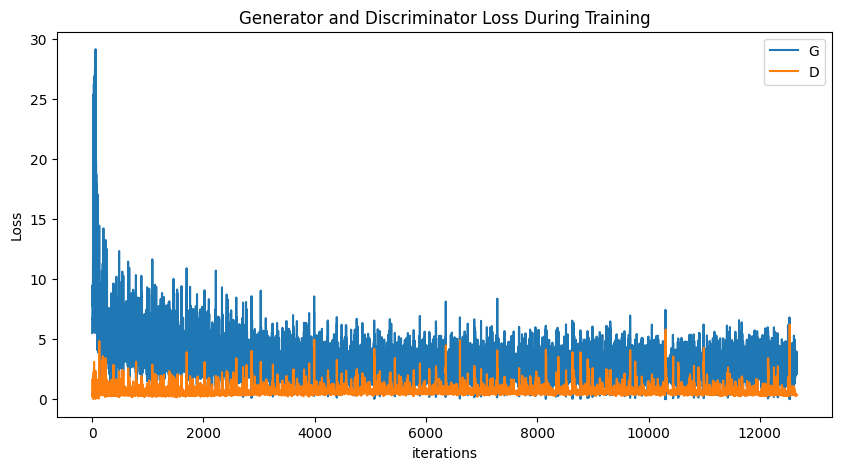
DCGAN Disciminator and Generator losses

Fig 8. DCGAN Disciminator and Generator losses.

The loss curves are somewhat intuitive. Initially the Generator is pretty bad, so its loss is high, but the strong gradient flow quickly brings its loss down to a level similar to Discirminator’s loss.

We can also display some final results from the Generator:

Generator outputs

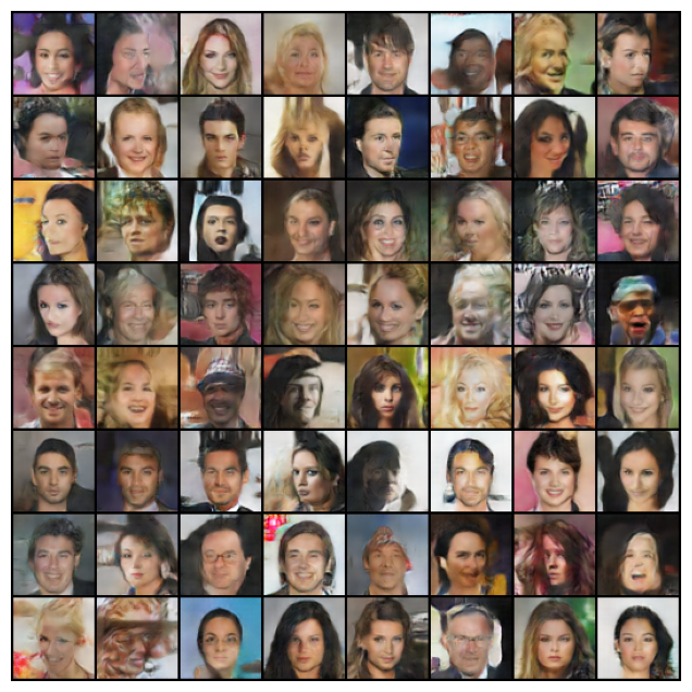
Fig 9. Generator outputs.

Performance

The DCGAN model measures its performance through a combination of qualitative and quantitative analyses. One common technique for evaluating the quality of unsupervised representation learning algorithms is to apply them as a feature extractor on supervised datasets and evaluate the performance of linear models fitted on top of these features. The authors train on Imagenet-1k and then use the discriminator’s convolutional features from all layers, maxpooling each layers representation to produce a 4 × 4 spatial grid. A regularized linear L2-SVM classifier is then trained on top to perform image classification on CIFAR-10 and the StreetView House Numbers dataset (SVHN). The classifier is able to achieve solid performance on both datasets, showing that the quality of unsupervised representation learning of DCGAN is good:

CIFAR-10 Benchmark

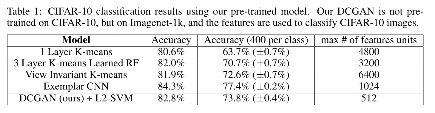
Fig 10. CIFAR-10 Benchmark.[2]

SVHN Benchmark

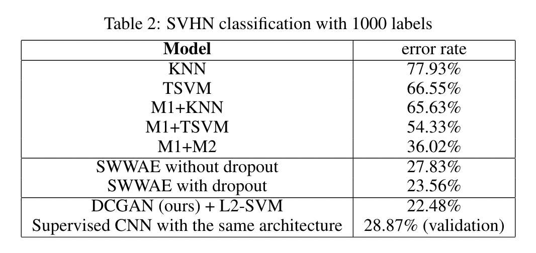
Fig 11. SVHN Benchmark.[2]

The authors further visualized DCGAN output and performed qualitative analysis on the internal of the networks. Full discussion can be found in the original paper.

Monet Style Transfer with CycleGAN

In this section, we will introduce CycleGAN and how to perform image style transfer using it. CycleGAN presents a framework for performing image-to-image translation in an unsupervised manner, i.e., without the need for paired examples in the training data. It’s particularly useful for tasks where collecting paired datasets is impractical. The innovation of CycleGAN lies in its ability to learn to translate between domains without direct correspondence between individual images, relying instead on the concept of cycle consistency.

Paired vs Unpaired Data

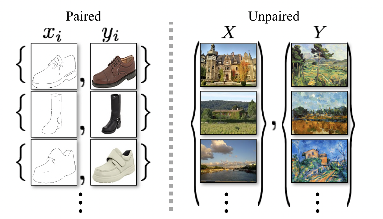
Fig 10. Paired vs Unpaired Data.[6]

How CycleGAN Works

CycleGAN utilizes two pairs of Generative Adversarial Networks (GANs), with each pair consisting of a generator and a discriminator. There are two generators, $G: X \rightarrow Y$ and $F: Y \rightarrow X$, where $X$ and $Y$ are two different image domains (e.g., horses and zebras). Each generator has a corresponding discriminator, $D_X$ and $D_Y$, which aim to distinguish between real and generated images in their respective domains.

CycleGAN Loss Function

The loss function of CycleGAN is composed of two major components: the adversarial loss and the cycle consistency loss. These components work together to ensure that the generated images not only belong to the target domain but also retain the key characteristics of the input images.

Adversarial Loss

The adversarial loss in CycleGAN functions similarly to that in traditional GANs, with the objective to make the generated images indistinguishable from real images in the target domain. The adversarial loss for generator $G$ and discriminator $D_Y$ is defined as:

\[\mathcal{L}_{\text{adv}}(G, D_Y, X, Y) = \mathbb{E}_{y \sim p_{\text{data}}(y)}[\log D_Y(y)] + \mathbb{E}_{x \sim p_{\text{data}}(x)}[\log(1 - D_Y(G(x)))]\]

And similarly, the adversarial loss for $F$ and $D_X$ is:

\[\mathcal{L}_{\text{adv}}(F, D_X, Y, X) = \mathbb{E}_{x \sim p_{\text{data}}(x)}[\log D_X(x)] + \mathbb{E}_{y \sim p_{\text{data}}(y)}[\log(1 - D_X(F(y)))]\]

Cycle Consistency Loss

The cycle consistency loss is defined as:

\[\mathcal{L}_{\text{cycle}}(G, F) = \mathbb{E}_{x \sim p_{\text{data}}(x)}[\|F(G(x)) - x\|_1] + \mathbb{E}_{y \sim p_{\text{data}}(y)}[\|G(F(y)) - y\|_1]\]

The cycle consistency loss plays a fundamental role in the CycleGAN framework by ensuring that the process of translating an image from its original domain $X$ to a new domain $Y$ and then back to $X$ results in an image that closely resembles the original. To understand how cycle consistency loss preserves original image features, consider the two parts of the cycle consistency loss formula:

$\mathbb{E}_{x \sim p_{\text{data}}(x)}[\|F(G(x)) - x\|_1]$ This term measures the difference between the original image $x$ from domain $X$ and the image that has been translated to domain $Y$ and then back to $X$ by the generators $G$ and $F$, respectively. The goal here is to minimize this difference, ensuring that the round-trip translation $F(G(x))$ results in an image that is as close as possible to the original $x$.
$\mathbb{E}_{y \sim p_{\text{data}}(y)}[\|G(F(y)) - y\|_1]$ Similarly, this term measures the difference between an original image $y$ from domain $Y$ and the image that has been translated to domain $X$ and then back to $Y$. The objective is to minimize this difference, which ensures that the cycle translation $G(F(y))$ preserves the content of the original image $y$.

By enforcing that images remain consistent through these round-trip translations, the cycle consistency loss effectively constrains the model to maintain the original content and features of the images while performing the domain translation.

Total Loss

The total loss for CycleGAN is a weighted sum of the adversarial and cycle consistency losses:

\[\mathcal{L}(G, F, D_X, D_Y) = \mathcal{L}_{\text{adv}}(G, D_Y, X, Y) + \mathcal{L}_{\text{adv}}(F, D_X, Y, X) + \lambda \mathcal{L}_{\text{cycle}}(G, F)\]

where $\lambda$ is a hyperparameter that controls the importance of the cycle consistency loss relative to the adversarial loss.

Architecture

CycleGAN utilizes established model architectures for the generators and discriminators. Both $G$ and $F$ use a series of convolutional layers for downsampling, a set of residual blocks for transformation, and convolutional layers for upsampling. Each generator translates an image from one domain to the other. For $D_X$ and $D_Y$, CycleGAN uses PatchGAN, which classify whether 70×70 overlapping patches are real or fake.

CycleGAN Generator Architecture

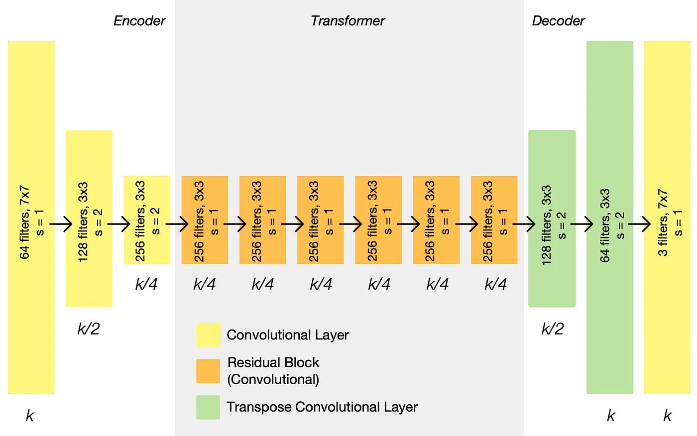
Fig 10. CycleGAN Generator Architecture.[7]

Implementation

Here, we present some high level implementations of CycleGAN. Code snippets are from a Kaggle notebook. Full notebook can be found here. Original code was written in TensorFlow. We implemented a Pytorch version instead.

Given two generators monet_generator and photo_generator and two discriminators monet_discriminator and photo_discriminator we can build a CycleGAN model as follows:

import torch
import torch.nn as nn
import torch.optim as optim
from torch.utils.data import Dataset, DataLoader
import torch.nn.functional as F

class ResidualBlock(nn.Module):
    def __init__(self, in_features):
        super(ResidualBlock, self).__init__()
        self.block = nn.Sequential(
            nn.Conv2d(in_features, in_features, kernel_size=3, stride=1, padding=1),
            nn.InstanceNorm2d(in_features),
            nn.ReLU(inplace=True),
            nn.Conv2d(in_features, in_features, kernel_size=3, stride=1, padding=1),
            nn.InstanceNorm2d(in_features)
        )

    def forward(self, x):
        return x + self.block(x)

class Generator(nn.Module):
    def __init__(self, input_channels, num_residual_blocks=9):
        super(Generator, self).__init__()
        # Initial convolution block
        model = [nn.Conv2d(input_channels, 64, kernel_size=7, stride=1, padding=3),
                 nn.InstanceNorm2d(64),
                 nn.ReLU(inplace=True)]
        # Downsampling
        in_features = 64
        out_features = in_features*2
        for _ in range(2):
            model += [nn.Conv2d(in_features, out_features, kernel_size=3, stride=2, padding=1),
                      nn.InstanceNorm2d(out_features),
                      nn.ReLU(inplace=True)]
            in_features = out_features
            out_features = in_features*2
        # Residual blocks
        for _ in range(num_residual_blocks):
            model += [ResidualBlock(in_features)]
        # Upsampling
        out_features = in_features//2
        for _ in range(2):
            model += [nn.ConvTranspose2d(in_features, out_features, kernel_size=3, stride=2, padding=1, output_padding=1),
                      nn.InstanceNorm2d(out_features),
                      nn.ReLU(inplace=True)]
            in_features = out_features
            out_features = in_features//2
        # Output layer
        model += [nn.Conv2d(64, input_channels, kernel_size=7, stride=1, padding=3),
                  nn.Tanh()]
        self.model = nn.Sequential(*model)

    def forward(self, x):
        return self.model(x)

class Discriminator(nn.Module):
    def __init__(self, input_channels):
        super(Discriminator, self).__init__()
        self.model = nn.Sequential(
            nn.Conv2d(input_channels, 64, kernel_size=4, stride=2, padding=1),
            nn.LeakyReLU(0.2, inplace=True),
            nn.Conv2d(64, 128, kernel_size=4, stride=2, padding=1),
            nn.InstanceNorm2d(128),
            nn.LeakyReLU(0.2, inplace=True),
            nn.Conv2d(128, 256, kernel_size=4, stride=2, padding=1),
            nn.InstanceNorm2d(256),
            nn.LeakyReLU(0.2, inplace=True),
            nn.Conv2d(256, 512, kernel_size=4, padding=1),
            nn.InstanceNorm2d(512),
            nn.LeakyReLU(0.2, inplace=True),
            nn.Conv2d(512, 1, kernel_size=4, padding=1)
        )

    def forward(self, x):
        return self.model(x)

The loss functions and CycleGAN Model can be implemented as:

class IdentityLoss(nn.Module):
    def __init__(self, lambda_identity=0.5):
        super(IdentityLoss, self).__init__()
        self.lambda_identity = lambda_identity
        self.loss = nn.L1Loss()

    def forward(self, real, same):
        return self.lambda_identity * self.loss(real, same)

class CycleGAN(nn.Module):
    def __init__(self, generator_X_to_Y, generator_Y_to_X, discriminator_X, discriminator_Y, device):
        super(CycleGAN, self).__init__()
        self.generator_X_to_Y = generator_X_to_Y
        self.generator_Y_to_X = generator_Y_to_X
        self.discriminator_X = discriminator_X
        self.discriminator_Y = discriminator_Y
        self.device = device

        self.adversarial_loss = AdversarialLoss().to(device)
        self.cycle_consistency_loss = CycleConsistencyLoss(lambda_cycle=10).to(device)
        self.identity_loss = IdentityLoss(lambda_identity=5).to(device)

The train loop can be implemented as following with necessary environment variables:

def train_cycle_gan(dataloader_X, dataloader_Y, cycleGAN, num_epochs=200):
    optim_G = torch.optim.Adam(
        list(cycleGAN.generator_X_to_Y.parameters()) + list(cycleGAN.generator_Y_to_X.parameters()),
        lr=0.0002, betas=(0.5, 0.999))
    optim_D_X = torch.optim.Adam(cycleGAN.discriminator_X.parameters(), lr=0.0002, betas=(0.5, 0.999))
    optim_D_Y = torch.optim.Adam(cycleGAN.discriminator_Y.parameters(), lr=0.0002, betas=(0.5, 0.999))

    for epoch in range(num_epochs):
        for batch_X, batch_Y in zip(dataloader_X, dataloader_Y):
            real_X = batch_X.to(cycleGAN.device)
            real_Y = batch_Y.to(cycleGAN.device)

            # Generators X->Y and Y->X
            fake_Y = cycleGAN.generator_X_to_Y(real_X)
            fake_X = cycleGAN.generator_Y_to_X(real_Y)

            # Generators' losses
            loss_G_X_to_Y = cycleGAN.adversarial_loss(cycleGAN.discriminator_Y(fake_Y), True)
            loss_G_Y_to_X = cycleGAN.adversarial_loss(cycleGAN.discriminator_X(fake_X), True)

            # Cycle consistency losses
            cycle_X = cycleGAN.generator_Y_to_X(fake_Y)
            cycle_Y = cycleGAN.generator_X_to_Y(fake_X)
            loss_cycle_X = cycleGAN.cycle_consistency_loss(real_X, cycle_X)
            loss_cycle_Y = cycleGAN.cycle_consistency_loss(real_Y, cycle_Y)

            # Identity losses
            identity_X = cycleGAN.generator_Y_to_X(real_X)
            identity_Y = cycleGAN.generator_X_to_Y(real_Y)
            loss_identity_X = cycleGAN.identity_loss(real_X, identity_X)
            loss_identity_Y = cycleGAN.identity_loss(real_Y, identity_Y)

            # Total generators' losses
            loss_G = loss_G_X_to_Y + loss_G_Y_to_X + loss_cycle_X + loss_cycle_Y + loss_identity_X + loss_identity_Y
            optim_G.zero_grad()
            loss_G.backward()
            optim_G.step()

            # Discriminators' losses
            real_X_loss = cycleGAN.adversarial_loss(cycleGAN.discriminator_X(real_X), True)
            fake_X_loss = cycleGAN.adversarial_loss(cycleGAN.discriminator_X(fake_X.detach()), False)
            loss_D_X = (real_X_loss + fake_X_loss) / 2

            real_Y_loss = cycleGAN.adversarial_loss(cycleGAN.discriminator_Y(real_Y), True)
            fake_Y_loss = cycleGAN.adversarial_loss(cycleGAN.discriminator_Y(fake_Y.detach()), False)
            loss_D_Y = (real_Y_loss + fake_Y_loss) / 2

            # Update discriminators
            optim_D_X.zero_grad()
            loss_D_X.backward()
            optim_D_X.step()

            optim_D_Y.zero_grad()
            loss_D_Y.backward()
            optim_D_Y.step()

            if batch_X == dataloader_X.dataset[-1]:
                print(f"Epoch {epoch+1}/{num_epochs}, Loss G: {loss_G.item()}, Loss D_X: {loss_D_X.item()}, Loss D_Y: {loss_D_Y.item()}")

CycleGAN Example Outputs

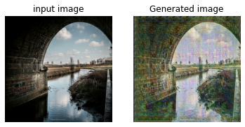
Fig 11. CycleGAN Example Outputs.[7]

Performance

The CycleGAN model is compared to several baseline models both quantitatively and qualitatively, using the same evaluation dataset and metrics as “pix2pix”.

Baseline models we used include CoGAN (learns one GAN generator for domain X and one for domain Y , with tied weights on the first few layers for shared latent representations), SimGAN (uses an adversarial loss to train a translation from X to Y), Feature loss + GAN (a variant of SimGAN where the L1 loss is computed over deep image features using a pretrained network), BiGAN/ALI (learn the inverse mapping function F : X → Z), and pix2pix.

First metric is AMT perceptual studies. This method involves “real vs fake” perceptual studies conducted on Amazon Mechanical Turk to evaluate the realism of the model’s outputs. Participants were shown pairs of images—one real and one generated by the algorithm—and asked to identify the real one. The studies aimed to assess the rate at which each algorithm could fool participants into thinking a generated image was real. The AMT performance table is shown in Figure 12.

CycleGAN AMT Metrics

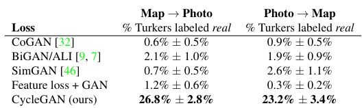
Fig 12. AMT “real vs fake” test on maps↔aerial photos at 256 × 256 resolution.[6]

Second metric is FCN Score. This automatic quantitative measure assesses how interpretable the generated photos are according to an off-the-shelf semantic segmentation algorithm (the fully-convolutional network, FCN). The FCN predicts a label map for a generated photo, which can then be compared against the input ground truth labels using standard semantic segmentation metrics. The intuition is that if a photo generated from a label map of a specific scene (e.g., “car on the road”) is successful, the FCN applied to the generated photo should detect the same scene elements. FCN scores table is shown in Figure 13.

CycleGAN FCN Score

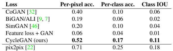
Fig 13. CycleGAN FCN Score.[6]

The last metric is Semantic segmentation metrics, which uses per-pixel accuracy, per-class accuracy, and mean-IoU to evaluate performance on Cityscapes photo to labels tasks. The performance table is shown in Figure 14.

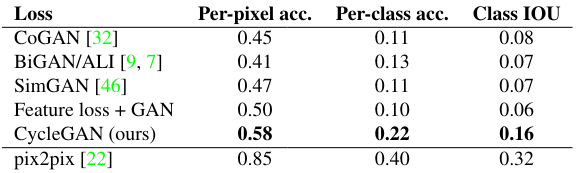
CycleGAN Semantic segmentation metrics

Fig 14. CycleGAN Semantic Segmentation Metrics[6]

From the above table we can see that CycleGAN outperforms all other baseline models on both subjective human judgment and objective machine-based metrics. These results shows that CycleGAN indeed has better performance and ability to generate indistinguishable images from the target images.

Text-to-image Generation with Imagen

In this section, we will discuss text-to-image generation with Imagen [8], one of the latest and best performing text-to-image models released by Google in December 2023. To enhance our understanding of such sophisticated models, we also explore simplified versions like MinImagen, which isolates Imagen’s salient features for educational purposes. This approach demystifies the complex technology, making it more accessible and providing a hands-on learning experience.

Imagen Architecture

Imagen first takes a textual prompt as the input and encodes it using a pre-trained T5 text encoder, which encapsulates the semantic information within the text. Imagen then feeds the encoding to the image generator, a diffusion model that starts with Gaussian noise and gradually denoise the image to generate a 64x64 small image as described by the textual prompt. Finally, the small image is upscaled by two super-resolution models (a type of diffusion model), generating a high-resolution 1024x1024 image as the output.

Imagen Architecture

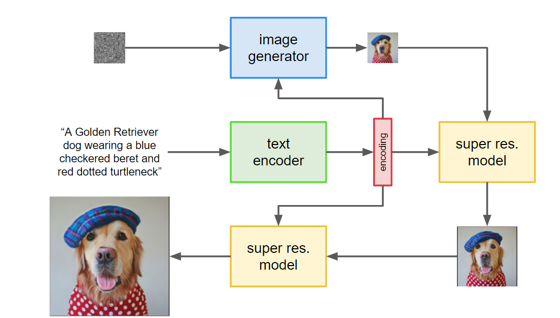
Fig 15. Imagen Architecture.[6]

T-5 text encoder

The T-5 text encoder (Text-to-Text Transfer Transformer) [10] is a general framework for NLP tasks released by Google in 2019. Unlike other text-to-image generation models like DALL-E 2, Imagen doesn’t use a text encoder explicitly trained on image-caption pairs. It is questionable that whether T-5 text encoder performs better than encoders specialized for text-to-image generation, but the overall performance of Imagen proves that T-5 works well.

T5 examples

Fig 16. T5 examples.[6]

One reason that contributes to the effectiveness of T-5 text encoder is its size [9]. Even though not trained on image-caption pairing tasks, the sheer size of extremely large language model still learns useful representation in text-to-text encoding task. One can argue that the size and quality of a model is more important than the specifics of the model itself.

U-Net architecture

The image generator in Imagen is a diffusion model, similar to other popular text-to-image models. One distinct feature of Imagen is to generate a low-resolution image in the middle of the entire workflow. However, diffusion model poses a restriction that its input and output must share the same dimensionalities and the image size must remain the same during the diffusion process.

To counter this restriction, Imagen chooses the U-net architecture [11]. U-Net is made up of two parts: an encoder and a decoder. The encoder is a series of convolutional and pooling layers that gradually downsample the input image to extract features at multiple scales. The decoder mirrors the encoder but in reverse, focusing on upscaling the feature maps and restoring the spatial dimensions to reconstruct the original image size.

U-Net Architecture

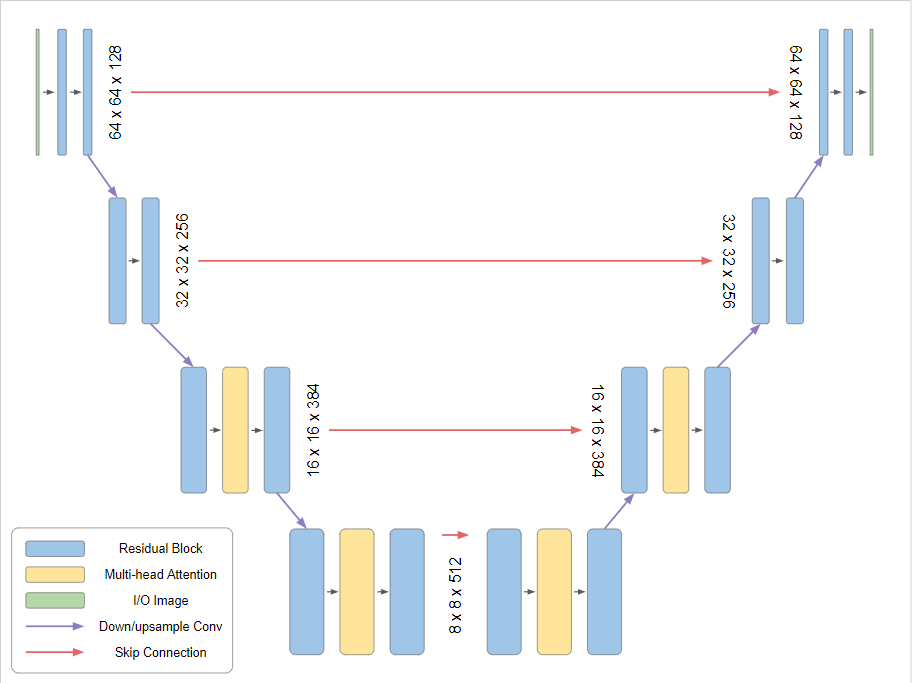
Fig 16. U-Net Architecture.[9]

Implementation of MinImagen in PyTorch

In this section, we detail the practical implementation of MinImagen, a simplified version of the Imagen model, using PyTorch. This implementation aims to provide a hands-on approach to understanding and working with text-to-image models by isolating Imagen’s core features.This approach demystifies the complex technology behind Imagen, making it more accessible and offering a practical, hands-on learning experience. The idea of simplifying such models for educational purposes aligns with efforts to make advanced AI techniques more approachable to a wider audience, as discussed in the MinImagen guide by O’Connor [12].

Step 1: GaussianDiffusion Class

The GaussianDiffusion class orchestrates the diffusion process, crucial for transitioning from noise to images in the generation process. This class handles the gradual addition and removal of noise over a predefined number of steps, utilizing a set variance schedule.

import torch
import torch.nn as nn


class GaussianDiffusion(nn.Module):
    def __init__(self, beta_start=0.0001, beta_end=0.02, timesteps=1000):
        super(GaussianDiffusion, self).__init__()
        self.beta_start = beta_start
        self.beta_end = beta_end
        self.timesteps = timesteps

        betas = torch.linspace(beta_start, beta_end, timesteps)
        alphas = 1.0 - betas
        alphas_cumprod = torch.cumprod(alphas, dim=0)

        self.register_buffer('betas', betas)
        self.register_buffer('alphas', alphas)
        self.register_buffer('alphas_cumprod', alphas_cumprod)
        self.register_buffer('sqrt_alphas_cumprod', torch.sqrt(alphas_cumprod))
        self.register_buffer('sqrt_one_minus_alphas_cumprod', torch.sqrt(1.0 - alphas_cumprod))

    def q_sample(self, x_start, t, noise=None):
        """
        Sample x_t from x_0 using the variance schedule.
        """
        if noise is None:
            noise = torch.randn_like(x_start)

        # Compute the noisy sample x_t at time t
        factor = self.sqrt_alphas_cumprod[t]
        x_t = x_start * factor + noise * torch.sqrt(1.0 - factor * factor)
        return x_t

    def q_posterior_mean_variance(self, x_start, x_t, t):
        """
        Compute the mean and variance of the reverse process posterior q(x_{t-1} | x_t, x_0).
        """
        posterior_mean = (
            self.sqrt_alphas_cumprod[t] * x_start +
            (1 - self.sqrt_alphas_cumprod[t]) * x_t
        )
        posterior_variance = 1 - self.sqrt_alphas_cumprod[t]
        return posterior_mean, posterior_variance

Step 2: Denoising U-Net

The Denoising U-Net plays a crucial role in predicting the noise at each diffusion step, facilitating the transition from noisy images back to clean images. This expanded example includes the encoder, bottleneck, and decoder sections with skip connections.

import torch
import torch.nn as nn
import torch.nn.functional as F

class ConvBlock(nn.Module):
    """A Convolutional Block consisting of Conv2D, Activation, and optional BatchNorm."""
    def __init__(self, in_channels, out_channels, kernel_size=3, stride=1, padding=1, use_bn=True):
        super(ConvBlock, self).__init__()
        self.conv = nn.Conv2d(in_channels, out_channels, kernel_size, stride, padding)
        self.activation = nn.ReLU(inplace=True)
        self.use_bn = use_bn
        if use_bn:
            self.bn = nn.BatchNorm2d(out_channels)

    def forward(self, x):
        x = self.conv(x)
        if self.use_bn:
            x = self.bn(x)
        x = self.activation(x)
        return x

class EncoderBlock(nn.Module):
    """Encoder block that reduces spatial dimensions by half and increases feature maps."""
    def __init__(self, in_channels, out_channels):
        super(EncoderBlock, self).__init__()
        self.conv_block = ConvBlock(in_channels, out_channels)
        self.downsample = nn.MaxPool2d(2)

    def forward(self, x):
        x = self.conv_block(x)
        x_downsampled = self.downsample(x)
        return x, x_downsampled

class DecoderBlock(nn.Module):
    """Decoder block that doubles spatial dimensions and reduces feature maps."""
    def __init__(self, in_channels, out_channels):
        super(DecoderBlock, self).__init__()
        self.upsample = nn.ConvTranspose2d(in_channels, out_channels, kernel_size=2, stride=2)
        self.conv_block = ConvBlock(in_channels, out_channels)

    def forward(self, x, skip_connection):
        x = self.upsample(x)
        x = torch.cat((x, skip_connection), dim=1)
        x = self.conv_block(x)
        return x

class Unet(nn.Module):
    """Denoising U-Net model for predicting noise at each diffusion step."""
    def __init__(self, in_channels=3, features=[64, 128, 256, 512]):
        super(Unet, self).__init__()
        self.encoders = nn.ModuleList()
        self.decoders = nn.ModuleList()

        # Encoder pathway
        for feature in features:
            self.encoders.append(EncoderBlock(in_channels, feature))
            in_channels = feature

        # Decoder pathway
        for feature in reversed(features):
            self.decoders.append(DecoderBlock(feature*2, feature))

        # Bottleneck
        self.bottleneck = ConvBlock(features[-1], features[-1]*2)

        # Final layer to map to 3 output channels
        self.final_layer = nn.Conv2d(features[0], 3, kernel_size=1)

    def forward(self, x):
        skip_connections = []

        for encoder in self.encoders:
            x, x_down = encoder(x)
            skip_connections.append(x)
            x = x_down

        x = self.bottleneck(x)

        skip_connections = skip_connections[::-1]

        for idx, decoder in enumerate(self.decoders):
            x = decoder(x, skip_connections[idx])

        x = self.final_layer(x)
        return x

Step 3: Integrating T5 Text Encoder

The T5 text encoder converts textual prompts into embeddings, guiding the image generation process. We utilize the transformers library to load a pre-trained T5 model.

from transformers import T5Tokenizer, T5ForConditionalGeneration
import torch.nn as nn

class TextEncoder(nn.Module):
    """
    This class utilizes the pre-trained T5 model from the Hugging Face transformers library
    to encode textual prompts into embeddings.
    """
    def __init__(self, model_name='t5-small'):
        """
        Initializes the TextEncoder with a specified T5 model.

        Parameters:
            model_name (str): Identifier for the Hugging Face model to be used.
        """
        super(TextEncoder, self).__init__()
        self.tokenizer = T5Tokenizer.from_pretrained(model_name)
        self.model = T5ForConditionalGeneration.from_pretrained(model_name)

    def encode(self, text):
        inputs = self.tokenizer(text, return_tensors="pt", padding=True, truncation=True, max_length=512)
        inputs = {k: v.to(self.model.device) for k, v in inputs.items()}  # Move inputs to the same device as model
        with torch.no_grad():
            outputs = self.model.encoder(**inputs)
        return outputs.last_hidden_state

Step 4: Training MinImagen

Training involves optimizing the model parameters to reduce the difference between the generated images and the target images. This process requires a dataset of text-image pairs.

import torch
import torch.nn as nn
import torch.nn.functional as F
from torch.utils.data import DataLoader, Dataset
from torchvision.transforms import Compose, ToTensor, Normalize, Resize
from torchvision.io import read_image
from pathlib import Path
import pandas as pd
import os
import torch.optim as optim
from transformers import T5Tokenizer, T5ForConditionalGeneration
from PIL import Image
import numpy as np

class MyDataset(Dataset):
    def __init__(self, root_dir, captions_file, transform=None):
        """
        root_dir (string): Directory with all the images.
        captions_file (string): Path to the text file with captions.
        transform (callable, optional): Optional transform to be applied on a sample.
        """
        self.root_dir = root_dir
        self.transform = Compose([
            Resize((256, 256)),
            Normalize(mean=[0.485, 0.456, 0.406], std=[0.229, 0.224, 0.225])
        ])
        self.captions_data = pd.read_csv(captions_file)
        self.images = self.captions_data['image']
        self.captions = self.captions_data['caption']

    def __len__(self):
        return len(self.captions_data)
    def __getitem__(self, idx):
        img_name = os.path.join(self.root_dir, 'Images', self.images.iloc[idx])
        if not os.path.exists(img_name):
            raise FileNotFoundError(f"Image file not found: {img_name}")

        image = read_image(img_name).float() / 255.0

        if self.transform:
            image = self.transform(image)

        caption = self.captions.iloc[idx]
        return caption, image

root_dir = '/content/drive/My Drive/archive'
captions_file = '/content/drive/My Drive/archive/captions.txt'

# Initialize the dataset and dataloader
transform = Compose([
    Normalize(mean=[0.485, 0.456, 0.406], std=[0.229, 0.224, 0.225])
])
dataset = MyDataset(root_dir=root_dir, captions_file=captions_file, transform=transform)
dataloader = DataLoader(dataset, batch_size=32, shuffle=True)


class MinImagenModel(nn.Module):
    def __init__(self, timesteps=1000):
        super(MinImagenModel, self).__init__()
        self.diffusion = GaussianDiffusion()
        self.unet = Unet()
        self.text_encoder = TextEncoder(model_name='t5-small')
        self.timesteps = timesteps

    def forward(self, text):

        # 1. Encode text to get text embeddings
        text_embeddings = self.text_encoder.encode(text)

        # 2. Generate initial noise
        noise = torch.randn(text_embeddings.size(0), 3, 256, 256, device=text_embeddings.device)

        # 3. Use the diffusion model and U-Net to transform the noise based on text embeddings
        for t in range(self.diffusion.timesteps):
            # Use the U-Net to predict noise and update the image tensor
            noise = self.unet(noise, text_embeddings)

        return noise
    def denoise_step(self, text_embedding, noise, t):
        # Predict the noise at timestep t
        noise_pred = self.unet(noise, t, text_embedding)

        # Retrieve necessary coefficients for denoising
        alpha_t, sigma_t = self.diffusion.coefficients(t)

        # Denoise the image using the predicted noise and coefficients
        denoised_image = (noise - sigma_t * noise_pred) / alpha_t

        return noise - 0.1 * noise


# Define 'device' to use GPU if available
device = torch.device('cuda' if torch.cuda.is_available() else 'cpu')

# Initialize the model and move it to the appropriate device
model = MinImagenModel().to(device)

# Define the optimizer using the optim module
optimizer = optim.Adam(model.parameters(), lr=0.001)

# Define the loss function
loss_fn = torch.nn.MSELoss()

model = model.to(device)
num_epochs = 10
for epoch in range(num_epochs):
    for batch_idx, (text, images) in enumerate(dataloader):
        images = images.to(device)  # Move images to the correct device

        # Convert text to embeddings and move to the GPU
        text_embeddings = model.text_encoder.encode(text).to(device)

        optimizer.zero_grad()
        predicted_images = model(text_embeddings)

        loss = loss_fn(predicted_images, images)
        loss.backward()
        optimizer.step()

        if batch_idx % 100 == 0:
            print(f'Epoch: {epoch+1}, Batch: {batch_idx}, Loss: {loss.item()}')

Step 5: Generating Images with MinImagen

After training, use the model to generate images from new text prompts.

import torch
from PIL import Image
import numpy as np

# Define the device
device = torch.device('cuda' if torch.cuda.is_available() else 'cpu')

# Define the function to generate the image
def generate_image(text_prompt, model, text_encoder, device='cuda'):
    model.eval()
    text_encoder.eval()

    # Encode text prompt to create text embeddings
    text_embedding = text_encoder.encode([text_prompt]).to(device)

    # Generate initial noise
    noise = torch.randn(1, 3, 256, 256, device=device)
    for t in reversed(range(model.timesteps)):
        noise = model.denoise_step(text_embedding, noise, t)

    # Convert the tensor to a PIL image
    generated_image = noise.squeeze().cpu().detach().numpy()
    generated_image = np.transpose(generated_image, (1, 2, 0))
    generated_image = (np.clip(generated_image, 0, 1) * 255).astype(np.uint8)
    pil_image = Image.fromarray(generated_image)

    return pil_image

# Initialize model and text_encoder instances
device = torch.device('cuda' if torch.cuda.is_available() else 'cpu')
model = MinImagenModel().to(device)
text_encoder = TextEncoder(model_name='t5-small').to(device)

text_prompt = "A scenic view of mountains at sunset"
generated_image = generate_image(text_prompt, model, text_encoder, device)
generated_image.show()

Imagen Performance

Quantitative performance

Using COCO, a dataset for evaluating text-to-image models, Imagen achieves a State-of-the-Art FID of 7.27 [8]. This outperforms DALL-E and even models that were trained on COCO, making Imagen one the best performing text-to-image models currently.

Qualitative performance

The authors of Imagen found that there are limitations in quantitative performance measurements like FID and CLIP. Instead, they perform qualitative assessment by using human subjects to evaluate the generated images. Each subject is shown 50 generated images, along with the ground-truth caption-image pairs from the COCO validation set.

To assess the quality of the generated images, the authors show each subject a generated image and its reference image and ask, “Which image is more photorealistic (looks more real)?” The resulted preference rate, where the subject chooses the generated image over the reference one, is 39.2%. [8]

To assess the image-caption alignment, the authors show each subject a generated image and its reference caption and ask, “Does the caption accurately describe the above image?” The subject can respond with “yes”, “somewhat”, and “no”, which corresponds to a score of 100, 50, and 0. The resulted alignment rate is 91.4, demonstrating a high level of congruence between the captions and the generated images. This qualitative assessment underscores Imagen’s ability to not only produce visually compelling images but also to ensure these creations are meaningfully aligned with their textual descriptions, highlighting the model’s nuanced understanding of language and visual representation. [8]

Reference

Please make sure to cite properly in your work, for example:

[1] Rombach, Robin, et al. “High-resolution image synthesis with latent diffusion models.” Proceedings of the IEEE/CVF conference on computer vision and pattern recognition. 2022.

[2] Radford, Alec, Luke Metz, and Soumith Chintala. “Unsupervised representation learning with deep convolutional generative adversarial networks.” arXiv preprint arXiv:1511.06434 (2015).

[3] Gatys, Leon A., Alexander S. Ecker, and Matthias Bethge. “A neural algorithm of artistic style.” arXiv preprint arXiv:1508.06576 (2015).

[4] Zhang, Lvmin, Anyi Rao, and Maneesh Agrawala. “Adding conditional control to text-to-image diffusion models.” Proceedings of the IEEE/CVF International Conference on Computer Vision. 2023.

[5] Li, D.-C.; Chen, S.-C.; Lin, Y.-S.; Huang, K.-C. A Generative Adversarial Network Structure for Learning with Small Numerical Data Sets. Appl. Sci. 2021, 11, 10823. https://doi.org/10.3390/app112210823

[6] Zhu, Jun-Yan, et al. “Unpaired image-to-image translation using cycle-consistent adversarial networks.” Proceedings of the IEEE international conference on computer vision. 2017.

[7] https://towardsdatascience.com/cyclegan-learning-to-translate-images-without-paired-training-data-5b4e93862c8d

[8] Saharia, C., Chan, W., Saxena, S., Li, L., Whang, J., Denton, E., Ghasemipour, S. K. S., Ayan, B. K., Mahdavi, S. S., Lopes, R. G., Salimans, T., Ho, J., Fleet, D. J., & Norouzi, M. (2022, May 23). Photorealistic text-to-image diffusion models with Deep Language understanding. arXiv.org. https://arxiv.org/abs/2205.11487

[9] O’Connor, R. (2022, October 18). How imagen actually works. Assembly AI. https://www.assemblyai.com/blog/how-imagen-actually-works/

[10] Roberts, A., & Raffel, C. (2020). Exploring transfer learning with T5: The text-to-text transfer transformer. Google Research. https://blog.research.google/2020/02/exploring-transfer-learning-with-t5.html?ref=assemblyai.com

[11] Nichol, A., & Dhariwal, P. (2021, February 18). Improved denoising diffusion probabilistic models. arXiv.org. https://arxiv.org/abs/2102.09672

[12] O’Connor, R. (2022, October 18). MinImagen: Build Your Own Imagen Text-to-Image Model. Assembly AI. https://www.assemblyai.com/blog/minimagen-build-your-own-imagen-text-to-image-model/