Mitigating Biases in Computer Vision
In this blog post, we investigate the issue of biases and model leakage in computer vision, specifically in classification tasks. We discuss traditional and deep learning approaches to prevent biases in classification models.
- Introduction
- Dataset Leakage and Model Leakage
- Classical Approach #1: Sample Weighing
- Classical Approach #2: Balanced Dataset
- Challenges of Classical Approaches
- Deep Learning Approach #1: Adversarial Debiasing
- Deep Learning Approach #2 Attribute-Orthogonal Detection
- References
Introduction
Trained computer vision classifier models reflects our own biases in society. For example, google baseball players and you will get pictures of almost all males. If you train a generative model to draw a person cooking in a home kitchen from Internet pictures, you are more likely to get a woman than a man. On the surface, these results come from unbalanced traning data. But the issue goes deeper than that. In the next few sections, we will discuss dataset leakage and model leakage, which result in biased behaviors of our models, classical approaches to correct biases, and two novel deep learning approaches.
We base our discussion on a few academic papers. See the reference section at the end of the blog.
Dataset Leakage and Model Leakage
To investigate the biases of our models, we need to first define two leakages: dataset leakage and model leakage. Dataset leakage measures the predictability of protected information, i.e. gender, from ground truth labels. Model leakage measures the predictability of protected information from model prediction.
A model is said to be amplifying biases if it exhibits stronger model leakage than dataset leakage.

Fig 1. Two women in a kitchen setting. Imbalanced datasets display strong dataset leakages. [1].
Now, let’s take a closer look at these two leakages.
Dataset leakage is defined as the the ability of an attacker f to successfully guess the protected information g based on the ground truth label Y. A dataset with, for example, overwhelming more female cooks than male cooks, can have a high level of dataset leakage.
\[\lambda_D = \frac{1}{|D|} \sum_{(Y_i,g_i) \in D} 1\{f(Y_i) == g_i\}\]Model leakage is similarly defined, except that the attacker f is guessing the protected information g based on the model prediction instead of the grounth truth label.
\[\lambda_M = \frac{1}{|D|} \sum_{(\hat{Y}_i,g_i) \in D} 1\{f(\hat{Y}_i) == g_i\}\]And finally, we define bias amplification to be the difference between model leakage and dataset leakage. It is to be expected for a model trained on imbalanced data to display large model leakage. What is even more concerning is that models tend to amplify biases, even when trained on balanced datasets.
\[\Delta = \lambda_M - \lambda_D\]Classical Approach #1: Sample Weighing
Given that we are working with inherently imbalanced datasets, i.e. high dataset leakage, one natural and simple approach is weighing the datapoints differently to balance out their probability of occurence. We adjust the weights to be the inverse of the degree of inclusion of their groups. For each ground truth i, assign the following weight:
\[w_i = \frac{\min_{g,a,s} P_{\text{tr}}(g, a, s)}{P_{\text{tr}}(g_i, a_i, s_i)}\]where \(g\), \(a\), \(s\) denote the gender, age, and skintone of the samples while \(P_{\text{tr}}\) denotes the distribution in the dataset.
We multiply the regression and classification loss of the weight \(w_i\) to penalize the model for making mistakes on minority datapoints.
Researchers at Amazon AI [2] ran an experiment using this approach using two variants of the RetinaFace face detector, one built on ResNet-50 and the other built on MobileNet-V1-0.25, and trained on the imbalanced WIDER FACE benchmark dataset. In both models, they demonstrated that compared to baseline results, weighted datasets showed a small bias reduction (Bias STD of 1.41 vs 1.46 on MobileNet and 1.11 vs 1.175 on ResNet).
Classical Approach #2: Balanced Dataset
The next intuitive step to mitigate bias is to construct a fully balanced dataset across protected datafields, such as gender, race, etc. Researchers at UCLA have done just that.
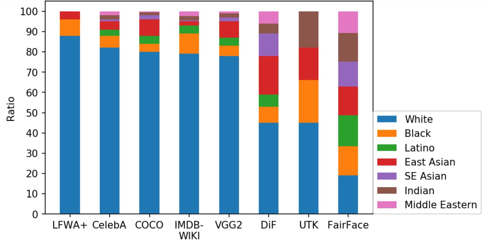
The FairFace dataset is formulated by Karkkainen and Joo at UCLA to be balanced across racial groups [3]. They first defined seven race groups: White, Black, Indian, Latino, East Asian, Southeast Asian, Latino, and Middle Eastern. They then collected images from the YFCC-100M dataset, which contains labels for race, age and gender. By construction, the FairFace dataset should suffer from little dataset leakage. We shall see if this alone is enough to train a perfectly fair model.
The final result is a dataset of roughly 100,000 faces. They found that models trained on their FairFace dataset performs better on novel datasets and have more balanced accuracies across race and gender.
Fig 2. Racial compositions of popular datasets. FairFace is balanced across race. [3].
Challenges of Classical Approaches
The most common challenge classical approaches face in regards to bias is unbalance data. Attempts have been made to address unbalanced datasets using sample weighing, but as discussed in the previous section, weighing the samples only shows a marginal improvement compared with baseline. The sample weighing approach is flawed. With datasets contraining very limited samples of one specific group, the weighing method tends to perform poorly.
Having balanced datasets alone isn’t perfect, either. Wang et al that even when they balanced training data so that
each gender co-occurred an equal amount of times with each target variable, the model still ampliied gender bias
as much as it did for unbalanced datasets. The researchers believe that this is due to the presence of features that are gender-correlated but unlabeled. For example, in a balanced dataset, if children are unlabeled but co-occur with the cooking action, a model could associate the presence of children with cooking. Since children co-occur with women more often than men, then model could then label women as cooking more often than expected. Because simply balancing the datasets has been shown to be an insufficient solution, novel deep-learning based approaches must be considered to mitigate bias in computer vision.
Deep Learning Approach #1: Adversarial Debiasing
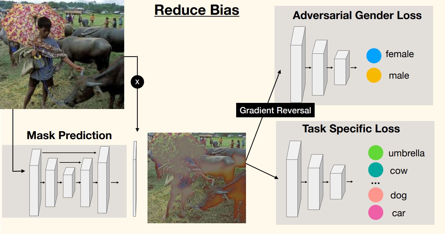
Since models trained on balanced datasets are not immune to amplifying bias, Wang et al then resorted to removing biases at the pixel level in training samples. To do this, they came up with Adversarial De-biasing to strategically apply a mask to pixels that give away protected information such as gender.
The adversarial part of this model comes in as a predictor and a critic. The critic is essentially a metric of model leakage; it tries to guess the protected information, in our case gender, from the class prediction of the predictor. The predictor acts the same as any classification model in the sense that it outputs a class based on the input image. The only difference in this case is that it also needs to maximize the critic’s loss, i.e. making it hard to guess the gender of the subject.
Fig 3. The Adversarial De-biasing model feeds the images through an encoder-decoder structure before training. [4].
To achieve the balacing act between the predictor and the critic, Wang et al employed a encoder-decoder network to process the image to censor the protected information. Essentially, this is analogous to a binary semantic segmentation task where the model needs to determine whether each pixel gives away protected information. Thus, the use of a encoder-decoder structure is intuitive.
Here is a look at the loss function; let’s look at it term by term.
\[L_p = \sum_i \left[ \beta |X_i - \hat{X}_i|_{\ell_1} + L(p(\hat{X}_i), Y_i) - \lambda L_c(c(\hat{X}_i), g_i) \right]\]The first term inside the summation notation is taking a \({\ell_1}\) norm between \(X_i\) and \(\hat{X}_i\). It is penalizing the model for making too much change to the original image, and thus encouraging the encoder-decoder to apply the minimal mask to censor the protected information.
The second term is the regular classification loss, where \(p\) refers to the predictor. After all, the model still needs to perform classification accurately.
The third term is the adversarial loss for the critic \(c\). Notice the negative sign. It is subtracting the critic’s loss, \(L_c\), from the total loss of the model. The worse the critic’s guesses are, the better the model is performing in bias mitigation. This is how the model removed explicit and implicit biases from the dataset.
The results are promising. Researchers have found model leakage has reduced over half while F1 score only decreased marginally. Such a decrease is reasonable since the mask takes away information from the training samples. More importantly, no one class suffers disproportinately.
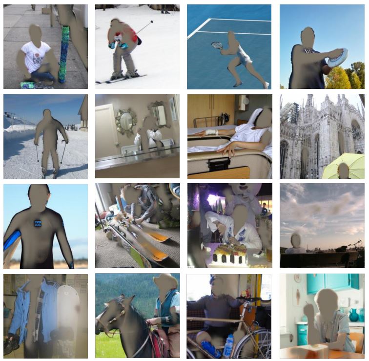
Taking a look at the mask the model applied reveals a interesting phenomenon. The model blurred out faces and body features that can give away the gender of the subject, while sparing the rest of the image. Some examples such as the tennis player and the skier are truly impressive.
Fig 4. Masks applied on training samples by Adversarial De-biasing Model. [4].
Deep Learning Approach #2 Attribute-Orthogonal Detection
However, Adversarial De-biasing inherently carries the risk of removing valuable information from the training samples, as demonstrated by the reduced accuracy. Also, it is expensive to solve the min-max problem required for the adversarial network.
To achieve better bias reduction than simply reweighing samples and to avoid using adversarial networks, researchers have come up with the Attribute-Orthogonal Detection method [1]. In this paper, the researchers attempt to mitigate the racial bias in face detection models.
Face detection models typically run a feature detector \(fe\) and a detector \(det\). The detector outputs bounding boxes and a classification from the feature map. It is trained on the bounding box regression loss \(L_{\text{reg}}\) and classification loss \(L_{\text{cls}}\).
Instead of an adversarial loss, this technique simply adds a regularization term to the network, similar to weight decay. But unlike weight decay, the Attribute-Orthogonal Detection regularizes the correlation between the parameters, \(\theta\), of the detector and the demographic classifier.
\[L_{\text{ortho}} = \frac{\|\theta_{\text{det}} \cdot \theta_{\text{cls}}\|_1}{\|\theta_{\text{det}}\|_2 \cdot \|\theta_{\text{cls}}\|_2}\]With the new regularization term, the final loss function becomes the following:
\[\min_{\theta_{\text{fe}}, \theta_{\text{det}}, \theta_{\text{cls}}} L_{\text{reg}} + L_{\text{cls}} + \alpha \ast L_{\text{ortho}}\]Essentially, it is encouraging the model to complete the detection and classification task independently, using weights as different as possible. This way, there is minimal correlation between how the model detects a face and classifies it. Thus, model leakage is minimized.
Notice that this method is far more lightweight than the adversarial method, though they are sharing the same goal.
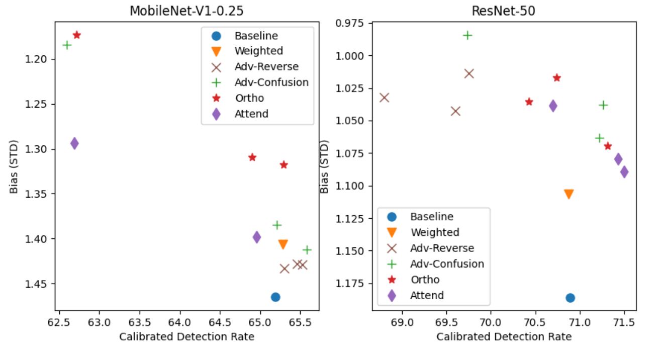
The results are promising. Here is a comparison of biases between models trained on different bias mitigation methods, such as sample weighing, adversarial, and attribute-orthogonal. The models are two variants of the RetinaFace architecture trained on the WIDER FACE dataset.
Fig 5. Attribute-Orthogonal Detection shows promising results. [2].
References
[1] https://www.istockphoto.com/photo/african-american-family-at-home-gm1371938299-441176461
[2] Yang, Gupta, et al. “Enhancing fairness in face detection in computer vision systems by demographic bias mitigation.” Proceedings of the 2022 AAAI/ACM Conference on AI, Ethics, and Society. 2022.
[3] Karkkainen, Kimmo, and Joo, Jungseock. “Fairface: Face attribute dataset for balanced race, gender, and age for bias measurement and mitigation.” Proceedings of the IEEE/CVF Winter Conference on Applications, 2021.
[4] Wang, Tianlu, et al. “Balanced Datasets Are Not Enough: Estimating and Mitigating Gender Bias in Deep Image Representations.” Proceedings of the IEEE/CVF International Conference on Computer Vision (ICCV). 2019, pp. 5310-5319.


