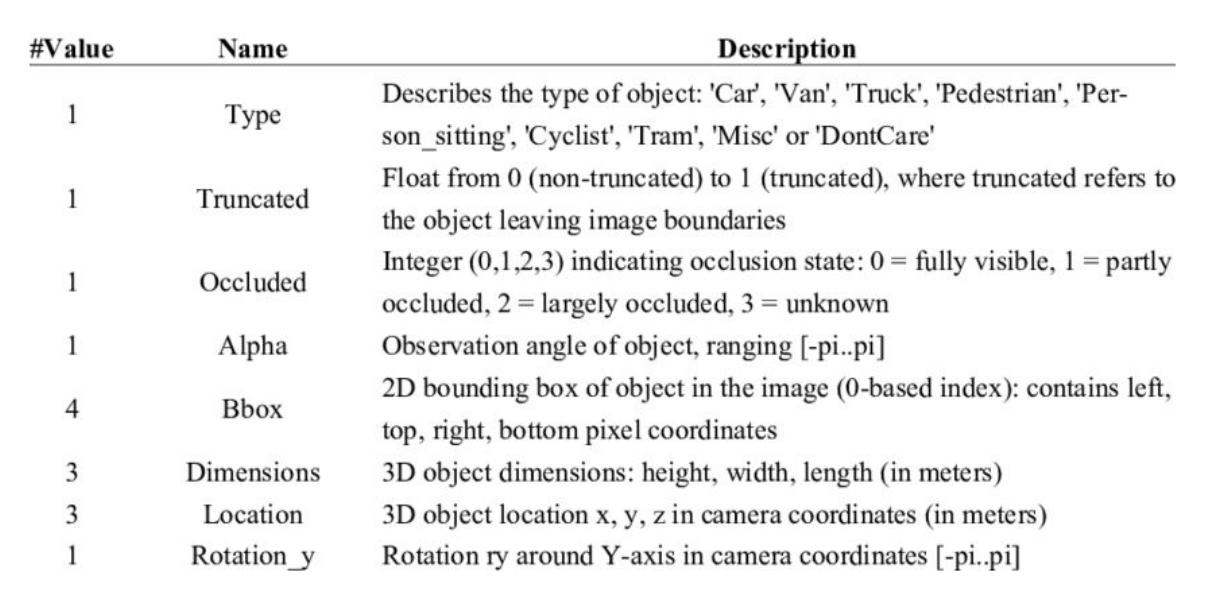
3d Bounding Box Estimation Using Deep Learning and Geometry
This blog delves into techniques for estimating 3d bounding boxes from monocular images, examining common datasets and evaluating three prominent methods. Additionally, it investigates enhancing the Deep3dBox model’s performance by incorporating temporal and stereo information, assessing the scalability of its geometric insights.
Introduction
3d object detection is a challenging task in computer vision where the goal is to identify and locate objects in 3d environments based on their shape, location and orientation. While there exists many multi-modal models that take advantage of different data from multiple sensors, the task of regressing 3d bounding box and orientation from monocular, 2D RGB images is a particularly challenging one.
In this final report, we explore different methods for 3d bounding box estimation from monocular images. We first briefly discuss about the common data set used to benchmark this task. Next, we analyze 3 different popular methods used and their pros and cons. Finally, we experiment with the Deep3dBox model by augmenting the amount of information available to the model by adding temporal information and stereo information and checking if the geometric insight of the original paper scaled.
Data Set
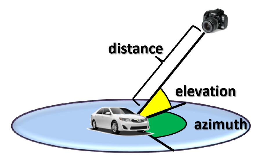
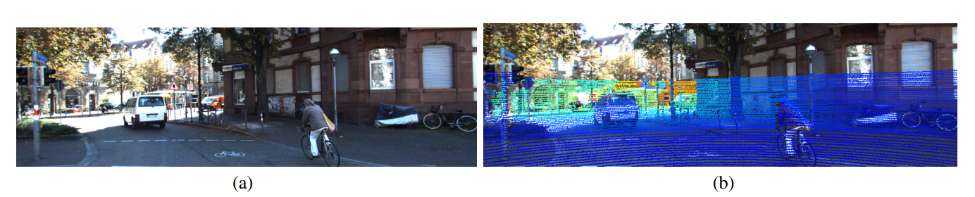
Most datasets consists of 2D images/videos that contain additional information such as Distance, Elevation, and Azimuth of the camera which is relevant for evaluating 3d Bounding box generated from 2D images/videos.
The additional information is often recorded in the form of point-clouds measured using LIDAR technology.
Alternatively, there are tools which can be used to map CAD models of objects onto 2d images.
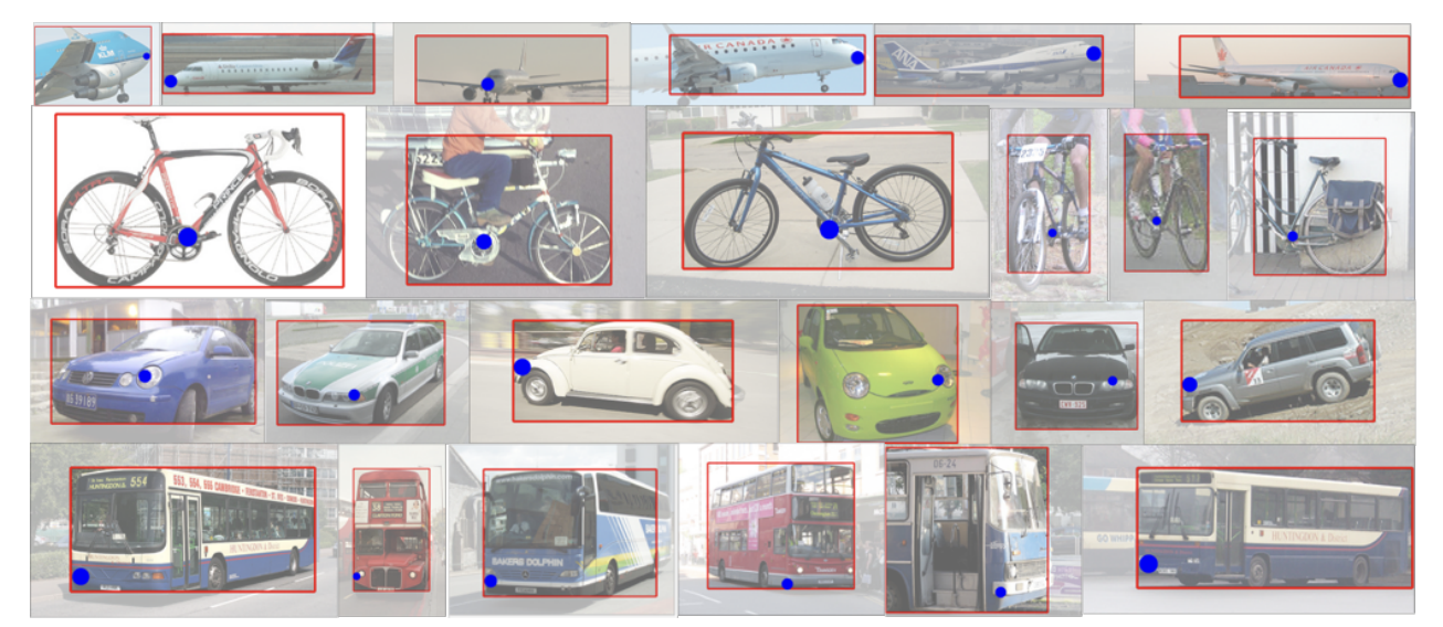
KITTI
One of the most popular benchmark dataset in 3d Object Detection is the KITTI dataset from 2012.
KITTI stands for Karlsruhe Institute of Technology and Toyota Technological Institute. The dataset includes: Various sensor modalities, High resolution RGB, 3d LIDAR data, GPS Localization data (tying objects to GPS coordinates).
For 3d Object detection, frames are selected to maximize the amount of cluttering objects There have been various work done by other researchers to label the data further.
The label processing is quite difficult, as labelling needs to be added on a pixel-wise and point-wise basis.
Metric for Evaluation: Orientation
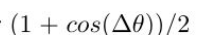
KITTI uses “Average Orientation Similarity”, which is calculated using the cosine similarity between predicted orientation and GT orientation. It is calculated using the alpha variable in the label.
In Deep3dBox, the loss function also uses the following criterion:
Models
Viewpoints and Keypoints
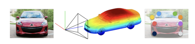
The paper “3d Bounding Box Estimation Using Deep Learning and Geometry” underscores the significances of pose estimation as it provides some critical information about the object’s orientation and position, by understanding the object’s pose, we can precisely determine its location, orientation relative to the observer. Another related work on pose estimation in particular is mainly introduced by the paper “Viewpoints and Keypoints”, it mainly characterizes the problem of pose estimation for rigid objects by separating it into two tasks - determining the viewpoint to capture the coarse overall pose, and predicting keypoints to capture the finer local details of the object’s configuration. It presents convolution neural network (CNN) based architectures to address both these tasks in two different settings. The first is a constrained setting where the bounding boxes around objects are provided, while the second is a more challenging detection setting where the goal is to simultaneously detect objects and estimate their pose correctly.
Method
1. Viewpoint Prediction
The authors formulate viewpoint prediction as a classification problem where the goal is to predict the three Euler angles (azimuth, elevation, and cyclo-rotation) corresponding to the object instance’s orientation. This is treated as a multi-class classification problem, where the potential angles is divided into bins, and a CNN is trained to classify each instance into one of these bins for each of the three angle types. The CNN architecture used is based on popular ImageNet models like AlexNet and VGGNet back in 2015, where they then applied transfer learning with the final layers reformulated for this multi-class angle classification task.
The key idea is that the hierarchical convolution layers can implicitly capture and aggregate local visual evidence across the image to predict these global orientation angles in an end-to-end fashion, without having to explicitly model part appearances or spatial relationships.
2. Keypoint Prediction
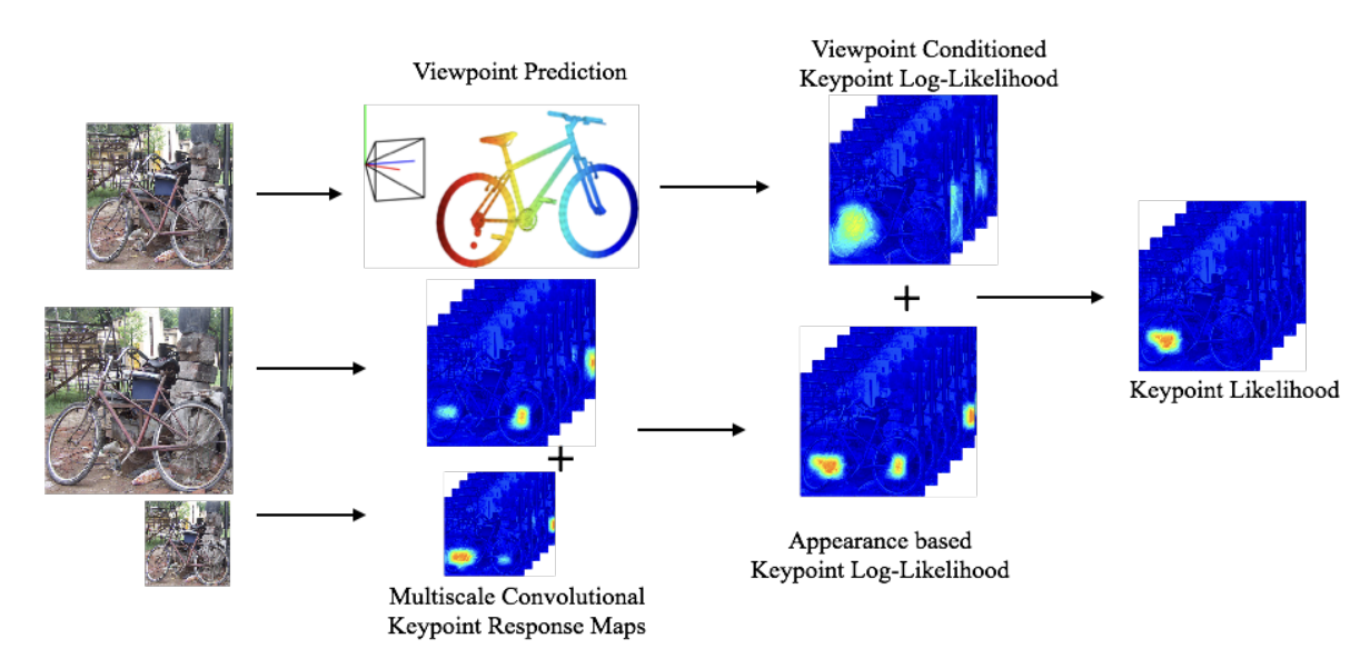
2.1 Multi-scale Convolutional Response Maps
For predicting keypoints like the positions of wheels, headlights etc., the authors propose modeling the local appearance of these parts using a fully convolutional CNN architecture. The network is trained such that the output feature maps correspond to spatial log-likelihood maps for the different keypoint locations. Specifically, the CNN contains convolutional layers borrowed from standard ImageNet architectures (follow similar approach as viewpoint prediction), followed by a final convolutional layer whose channels correspond one-to-one to the different keypoints being predicted across all object categories. During training, the target outputs are constructed as Gaussian response maps centered at the annotated keypoint locations.
To benefit from reasoning at multiple scales, the authors train two parallel CNNs - one at a higher 384x384 resolution capturing finer details, and another at a lower 192x192 resolution capturing some more context around each part.
2.2 Viewpoint Conditioned Keypoint Likelihood
In addition, while modeling local appearance is important for accurate keypoint localization, the global viewpoint context is also crucial to resolve ambiguities and predict likely keypoint configurations. For example, for a left-facing car, we expect the left wheel to be visible but not the right wheel based on the overall pose.
To incorporate this global viewpoint reasoning, they propose a non-parametric mixture model that represents the conditional probability distribution of each keypoint’s location given the predicted viewpoint. Specifically, for a test instance with predicted viewpoint R, they first retrieve all training instances whose viewpoint is within π/6 radians of R. Then the conditional keypoint likelihood is modeled as a mixture of Gaussian centered at the keypoint annotations from these retrieved instances.
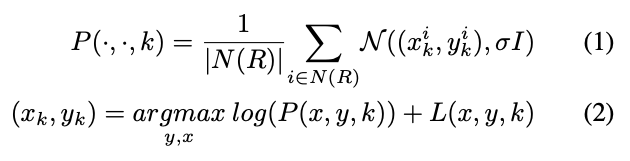
This viewpoint conditional likelihood is combined with the multi-scale appearance likelihood maps through a simple sum of log-likelihood scores, to produce the final keypoint location predictions as shown below.
Experiments and Results
1. Viewpoint Estimation
They first analyze viewpoint estimation performance in a constrained setting where ground-truth bounding boxes are provided. The metrics used are:
1) Median Geodesic Error: This measures the median geodesic distance between predicted and ground-truth rotation matrices across instances. It is robust to outliers.
2) Accuracy at θ threshold (Accθ): This measures the percentage of instances whose predicted viewpoint is within θ radians of the ground-truth.
Their CNN-based approach achieves a Mean Accπ/6 of 0.81 and Median Error of 13.6° across categories, significantly outperforming baseline methods that use linear classifiers on CNN features or explicit part modeling with deformable part models.
For the more challenging detection setting where bounding boxes are not provided, they use object proposals from selective search or region proposal networks. They evaluate using three metrics:
1) AVP: Originally proposed metric computing mAP for azimuth angle prediction only, within correct detections.
2) AVPθ: Their proposed metric extending AVP to compute mAP with a angle threshold θ.
3) ARPθ: Similar to AVPθ but accounts for errors in all three Euler angles.
Their method achieves an ARPπ/6 of 46.5%, significantly better than the previous state-of-the-art of 17.3%.
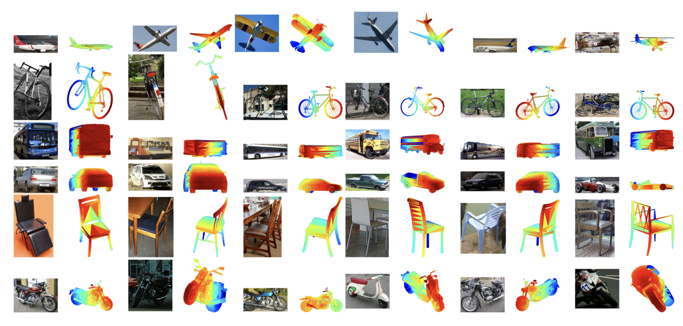
2. Keypoint Prediction
Keypoint Localization
In this setting, with ground-truth bounding boxes provided, the goal is to localize keypoints within visible object instances. They use the PCK metric, achieving a PCK of 68.8% at α=0.1.
Keypoint Detection
In this more challenging setting without bounding boxes, predictions are scored using precision-recall curves, with APK used as the metric. Their method achieves a mean APK of 33.2% at α=0.1 threshold across categories.
They also evaluate on articulated human pose estimation, achieving an APK of 0.22 on PASCAL, outperforming specialized state-of-the-art methods.
Analysis
Pros
The key strengths of the proposed method are:
-
By using an end-to-end trained convolutional architecture, it avoids the need for explicit modeling of part appearances or deformations, letting the CNN implicitly learn the relevant representations.
-
It presents a principled approach to combine local appearance cues with global viewpoint context for improving keypoint predictions.
Cons
Some potential limitations of the work are:
-
While avoiding explicit part modeling is a strength, the proposed method still relies on the discriminative power of the CNN architecture. It lacks explicit 3d geometric reasoning which could be beneficial.
-
The experiments and analysis are restricted to rigid object categories like vehicles, furniture etc. The applicability to non-rigid or highly articulated objects like animals is not evaluated.
-
While incorporating viewpoint improves over pure appearance models, precise localization of keypoints with high accuracy remains a challenge based on the PCK/APK numbers reported.
Comparison
Applicability and Generalization
“Viewpoints and Keypoints”: The method is primarily evaluated on rigid objects like vehicles and furniture. It may face limitations in generalizing to non-rigid or highly articulated objects due to its focus on specific object categories and tasks.
“3D Bounding Box Estimation Using Deep Learning and Geometry”: The approach is applicable to a wide range of objects, including both rigid and non-rigid objects. It offers potential advantages in scenarios where accurate geometric models are crucial for accurate 3D bounding box estimation.
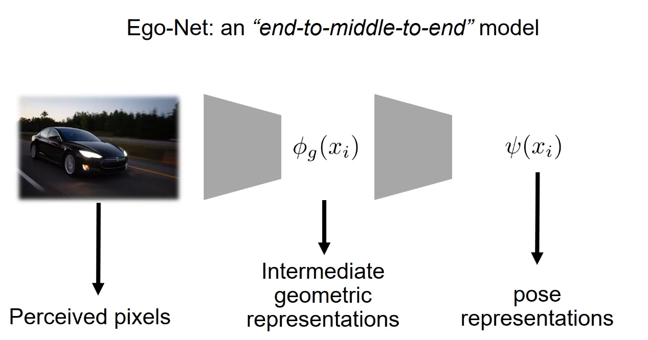
Intermediate Geometric Representation Based Method: Ego-Net
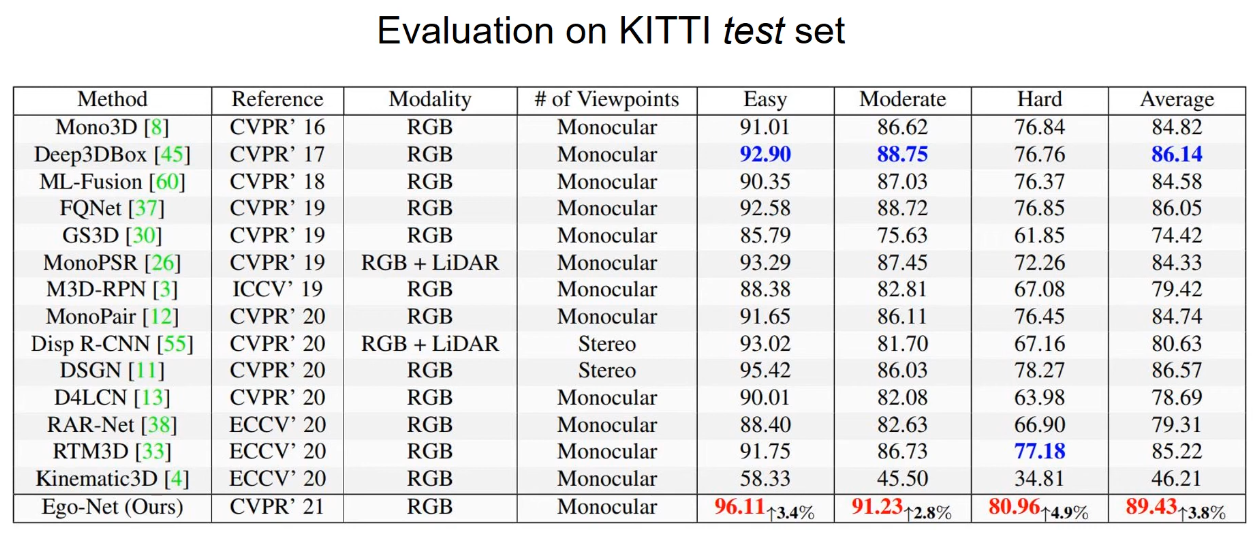
Another popular method of regressing 3d pose from 2d images is through the extraction of intermediate geometric representation. The best performing model of this class is the Ego-Net from 2021 [2]. This class of model is also similar to Deep3dBox, as they both try to regress 3d pose from 2d images.
IGR
Inspired by the representational framework of vision introduced by Marr, Ego-Net explicitly defines and coerces the model to first learn some intermediate geometric representations.
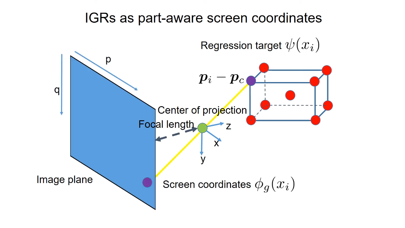
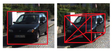
IGR Regression target
The model attempts to regress the orientation relative to the center of a cuboid. The regressed, correctly oriented cuboid is then projected back to the image plane. The 2D coordinate of the projection is the desired IGR.
Custom Loss Function
The lost function used for this model consists of heatmap, 2d and 3d loss.
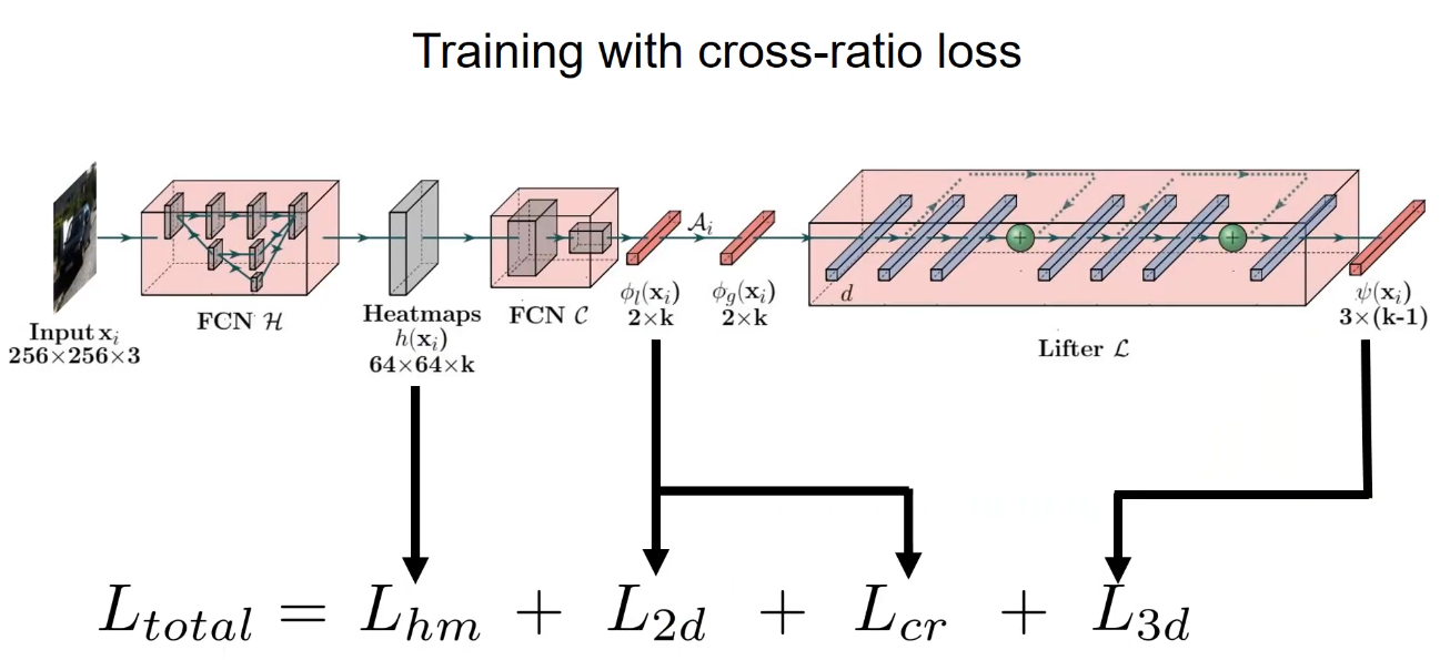
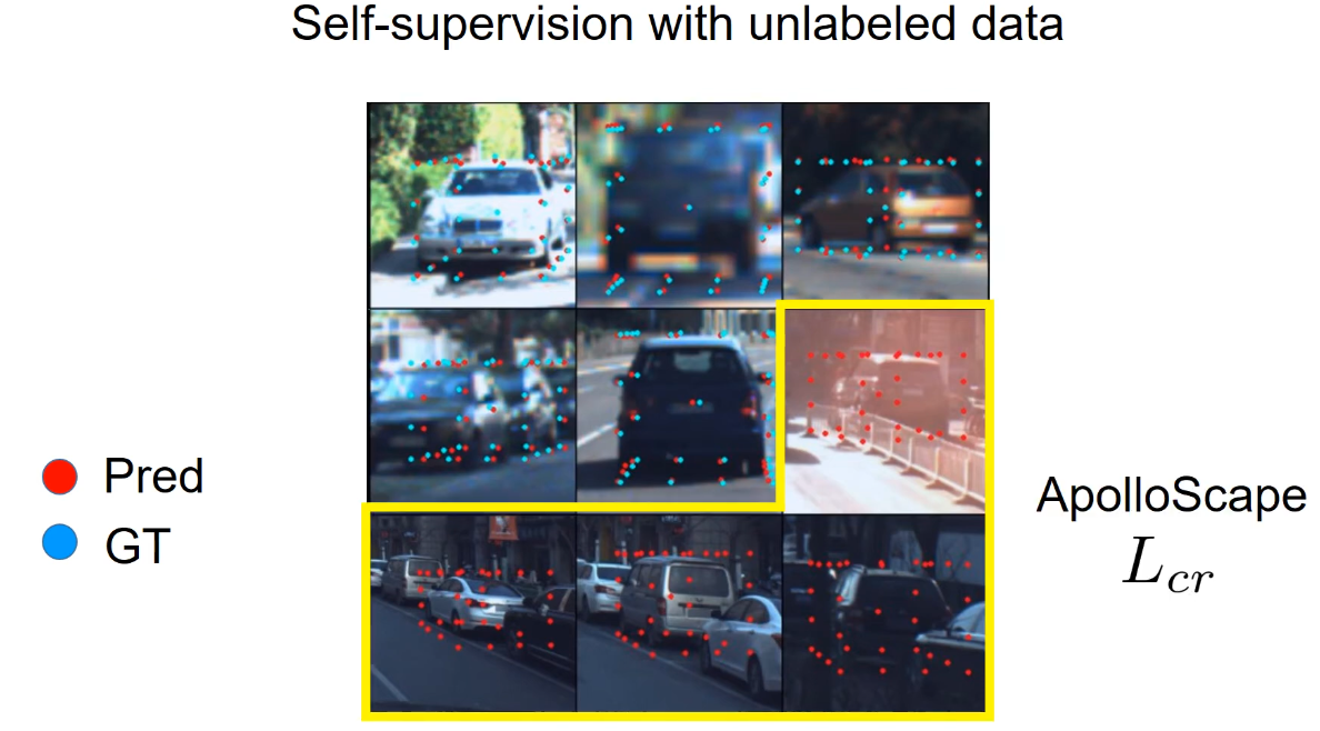
Another novel loss used in Ego-Net is cross ratio loss function.
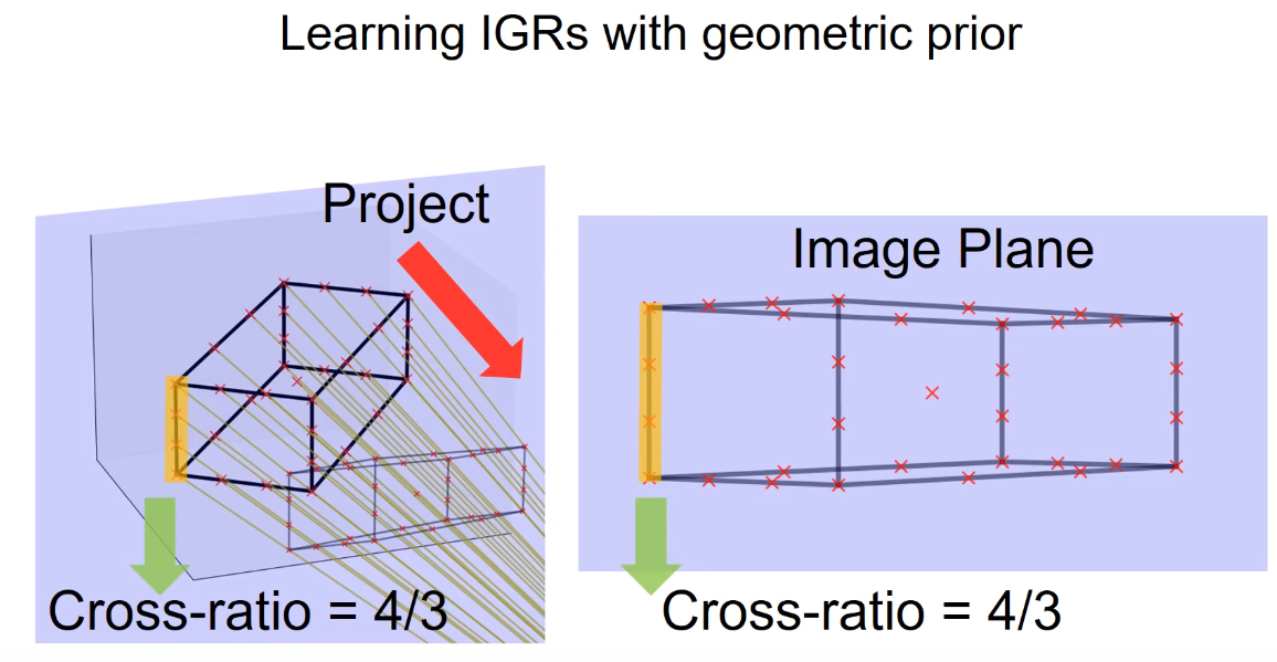
Since cross ratio is a projection invariant, the IGR’s cross-ratio should be the same as the predicted 3d bound boxes’ cross ratio.
The use of the cross ratio loss function allows for self-supervised learning using only the cross ratio loss without a 2d ground truth.
Analysis
Many previous models attempt to directly map 2d pixels to angular representation of 3d poses. The drawbacks of these previous models is that local appearance alone in a 2d image is not sufficient to determine vehicle pose.
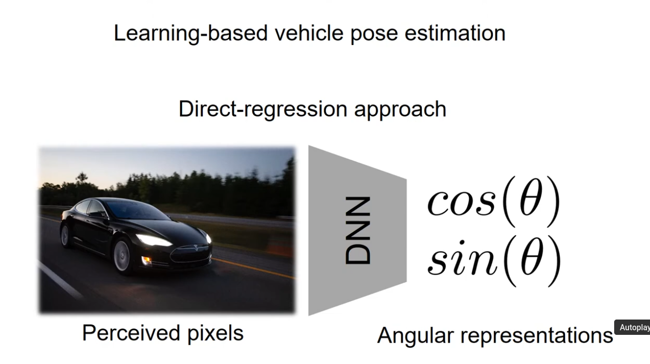
Furthermore, extracting 3d pose directly from 2d pixels is a highly non-linear and difficult problem.
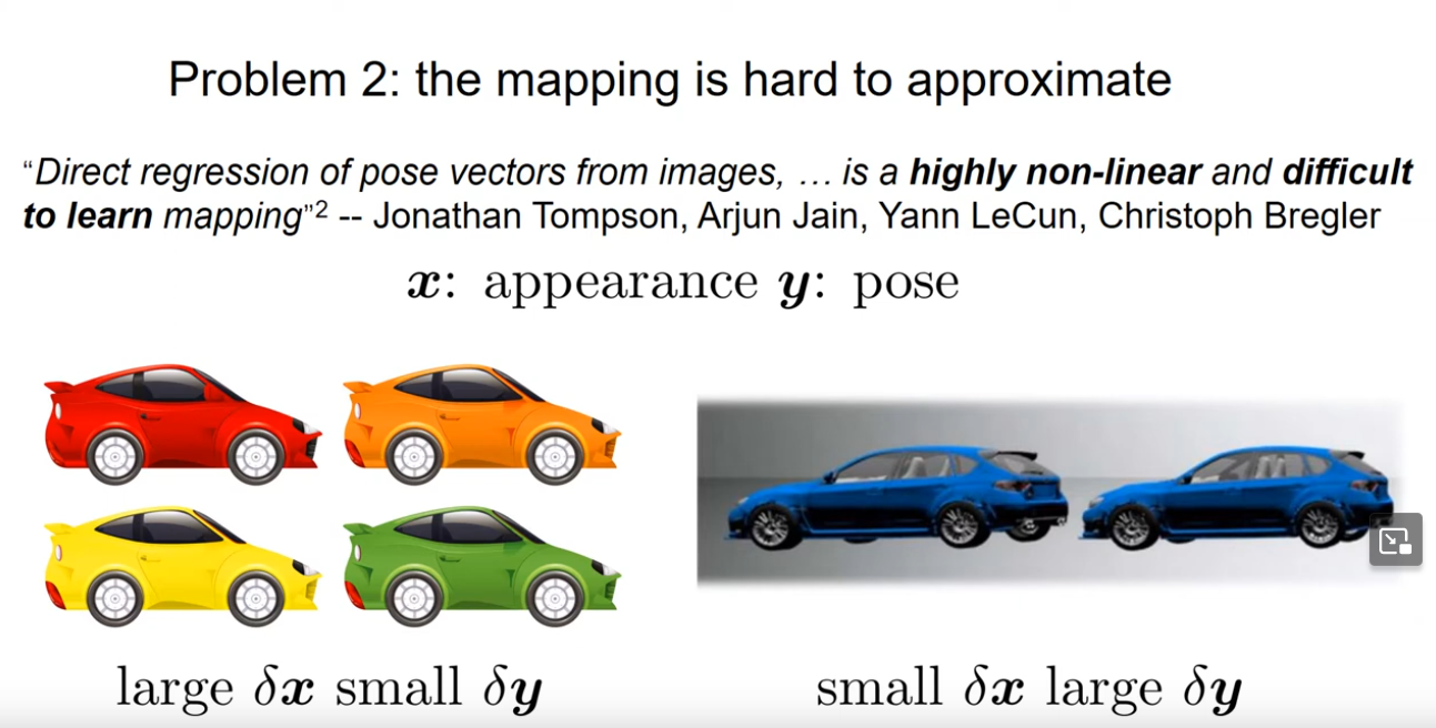
Thus, by using IGR, Ego-net is able to achieve better results by reducing the difficulty of the regression problem with a useful intermediate representation.
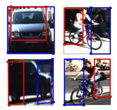
3d Bounding Box Estimation based Method: Deep3dbox
“3d Bounding Box Estimation Using Deep Learning and Geometry, Mousavian et al. 2017”[4]. starts with a 2D bounding box, and estimates 3d dimensions/orientation using that.
The model utilizes a Hybrid discrete-continuous loss function Geometric constraints from 2D bounding box for training.
The model’s primary goal is to attempt to regress 3d Object Dimensions from 2d bounding boxes. As a part of the loss function,
3d Dimension Regression
One of the first goals of the model is to regress 3d object dimensions from the 2d bounding boxes.
The model makes the assumption that the 2d bounding boxes provided by the model is as tight as possible, and each side of the 2d box touches the projection of 1 or more of the 2d box’s corners.
With these assumptions in mind, the model attempt to derive a set of mathematical constraints through coordinate projection.
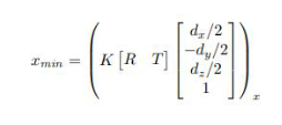
To do the actual regression for bounding box, the model uses a network of CNNs. After successfully regressing the bounding box, the model attempts to find the center point T of the bounding box that minimizes re-projection error.
Some simplifying assumptions made about the model is that it is upright, and that there is no roll or pitch.
Multibin CNN Module
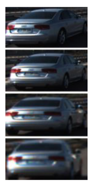
3d Orientation must be understood in the context of local orientation \(\theta_l\) and camera angle \(\theta_c\).
In the images below, the global orientation doesn’t change, even though the camera view changed. We thus try to regress \(\theta_l\).
To take advantage of existing models, the Multibin CNN module is added onto a pre-trained VGG network [5]. Orientation angle is discretized into several possible bins. Estimate confidence that true angle belongs in each bin (column 3), necessary correction to θ ray (column 2), and dimensions based on the ITTI object category (column 1). Bin with max. confidence is selected during inference
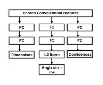
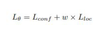
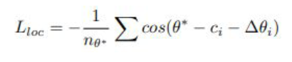
Multi bin Loss Function
Orientation Loss:
Localization Loss:
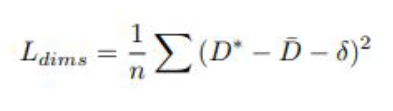
Dimension Loss:
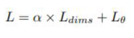
Total Loss:
Analysis
Some novel aspects of this method are its advanced cropping feature which allows the FC layers to focus on determining orientation rather than trying to identify cars and its novel loss function which is utilize cosine difference.
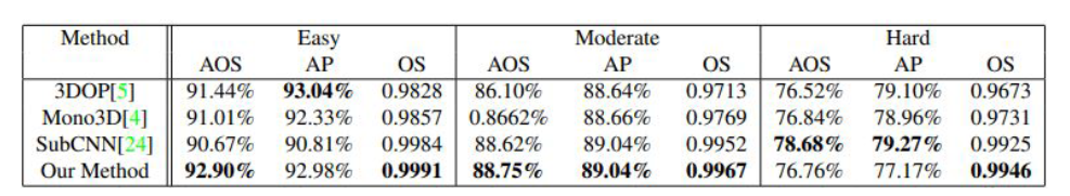
The model was able to beat stereo/semantic segmentation models thanks to its clever geometric insights. It was able to achieve:
-
1st place for Average Orientation Estimation, Average Precision on KITTI Easy/Moderate datasets
-
1st place on KITTI Hard in Orientation Score (excludes 2D bounding box estimation)
-
Beats SubCNN in other metrics (e.g. 3d box IoU) 3-8 deg of orientation error across KITTI Easy/Moderate/Hard
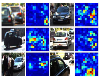
The model was also able to demonstrate the “Attention” where it focuses on features such as tires and mirrors to determine orientation.
Methods
Deep3dbox was highly successful in mono 3d pose estimation by use of clever geometric insights. We were interested to see if these geometric insights scaled, and experimented with augmenting it with both temporal information(the last 3 frames) and stereo information(right camera). To study this, we created an extensible framework which increased the information given to the model without compromising the models fundamental architecture.
Preprocessing
Deep3dbox requires that each the image be cropped to its bounding box. As a result, extending this model to more information requires nontrivial preprocessing decisions. These are presented in diagram from below.

In words, each of the images are extracted from their file, then compared against the ground truth labels to find the location of the bounding boxes. These images are then cropped to their bounding box, normalized, and concatenated. We chose the convention that stereo images would be concatenated horizontally, while temporal images would be concatenated vertically. It should also be noted that each image was cropped to the points given in the baseline “mono” image. This was done for several reasons:
- Keeping the points the same can increase temporal information. As an example, picture a car driving perpendicular to the camera. Changing the crop location would make the previous frames almost identical to the current frame, giving no extra information. Cropping from the same location allows the car to move in the cropped image, communicating movement to the neural net.

-
Deep3dBox is heavily based on estimating the local orientation angle, so there were concerns about introducing multiple global angles to the problem.
-
KITTI only seems to provide these labels for the left camera at the frame of annotation.
Neural Net Architecture
Deep3dBox is relatively size agnostic, but did require some tweaking to work with larger input sizes. Like the paper, our initial feature space is created by VGGNet’s convolution layers, so nothing needs to be done there. However, all three neural nets(dimensions, orientation, and confidence) begin with a fully connected layer from this feature space into the embedding. To keep the architecture similar to the paper, we chose to increase the input size of this linear layer, and keep the architecture of the other layers exactly the same from run to run.
The above decision results in the total parameters increasing for models with more data, which requires increased training time and increases the flops per forward pass. To make sure the project was still completable under limited compute resources, max pooling with a kernel of size (4,2) and stride (4,2) was implemented between VGGNet and the linear networks on the stereo-temporal architecture.
Training
All networks were trained with SGD with momentum=0.9, and used a batch size of 10. Networks were trained for 20 epochs, except for mono-temporal and stereo. To account for the additional parameters seen in mono-temporal and stereo, they were given 30 epochs to train. Stereo-temporal was not given these 10 extra epochs due to compute time constraints and the max pooling used to reduce the parameter space.
It should also be noted that each model required drastically different amounts of training time. Unfortunately, this was not tracked precisely, as this level of variance was not expected. Rough numbers are available below.
| Model | Training Time | Num Epochs | Reason |
|---|---|---|---|
| Mono | 10 Hours | 10 | Recommended value in other projects |
| Stereo | 16 Hours | 20 | More parameters |
| Mono, last 3 frames | 1 Day | 30 | More parameters |
| Stereo, Last 3 Frames | 2 Days | 20 | Compute time constraints only allowed training for 20 epochs |
While some of this is due to the inefficiency in concatenation and preparing the forward pass, it suggests that VGGNet and the increased size linear layers increase the time of the forward and backward pass. This is a concern for self driving vehicles, where 3d bounding box information needs to be available in real time.
Validation and training were split by whether the last digit of the id ended in 9. This resulted in 10% of the data being reserved for validation.
Discussion
Temporal and Stereo infusion results
After training for a variable number of epochs, we obtained the results below
| Model | Mean IoU | Std IoU | Mean Angle Difference (rad) | Std Angle Difference (rad) |
|---|---|---|---|---|
| Stereo temporal | 0.956 | 0.00023 | -0.0037 | 0.2515 |
| Mono temporal | 0.983 | 0.00059 | -0.0087 | 0.2229 |
| Stereo | 0.993 | 0.00026 | -0.0338 | 0.1167 |
| Baseline | 0.992 | 0.0012 | 0.0003 | 0.1439 |
Notably, all models were able to perform dimension size vehicle estimation with high precision, with an IoU of effectively 1. However, these models exhibit high differences in orientation prediction. While models exhibit a mean angle difference close to ground truth, including temporality appears to double standard deviation in angle difference. This implies the model exhibits poor training performance when provided with temporal data, which could be an indication of several things:
- Pose estimation does not require temporal data, so adding it effectively adds noise to the linear network
- The increased number of inputs to the first linear network increases the parameter count, requiring quadratically more training time rather than the linear increase that was given.
- The architecture performs poorly with downsampling, which was required in the stereo temporal model.
However, stereo vision without temporal data resulted in an 18.9% decrease in Std. angle difference, which implies that stereo vision greatly assists with pose estimation. This makes sense, as stereo vision gives the model access to parallax, which increases its ability to judge depth and determine angle.
IGR based methods would likely also benefit from stereo vision without temporal data, since it would make minimizing the cross ratio loss easier.
Finally, it’s worth noting that our baseline model has roughly the same angle deviation as seen in the paper, which is a good indication these results stem purely from architecture, and not choice of optimizer or hyperparameter.
Reference
[1] Redmon, Joseph, et al. “You only look once: Unified, real-time object detection.” Proceedings of the IEEE conference on computer vision and pattern recognition. 2016.
[2] Shichao Li and Zengqiang Yan and Hongyang Li and Kwang-Ting Cheng, et al. “Exploring intermediate representation for monocular vehicle pose estimation” CVPR. 2021.
[3] S. Tulsiani and J. Malik. Viewpoints and keypoints. In CVPR, 2015.
[4] A. Mousavian, D. Anguelov, J. Flynn and J. Košecká, “3D Bounding Box Estimation Using Deep Learning and Geometry,” 2017 IEEE Conference on Computer Vision and Pattern Recognition (CVPR), Honolulu, HI, USA, 2017, pp. 5632-5640, doi: 10.1109/CVPR.2017.597. keywords: {Three-dimensional displays;Two dimensional displays;Solid modeling;Pose estimation;Object detection;Shape},
[5] K. Simonyan and A. Zisserman, in 3rd International Con- ference on Learning Representations, ICLR 2015, San Diego, CA, USA, May 7-9, 2015, Conference Track Pro- ceedings, edited by Y. Bengio and Y. LeCun (2015). —