Anomaly Detection for Semantic Segmentation
When semantic segmentation models are used for safety-critical applications such as autonomous vehicles, they have to handle unusual things that don’t fall into one of the predefined categories that they were trained for. We discuss two state-of-the-art methods that attempt to detect and localize anomalies, one using kNN and the other using generative normalizing flow models.
Introduction
Semantic segmentation models take an image as input and classify each pixel. One application of these models is autonomous vehicles, where a model might take images from a front-facing camera and determine whether pixels correspond to the road, other vehicles, etc. These models are typically designed to output a fixed set of classes, but when they are deployed in the real world, they will inevitably encounter unusual things that don’t fall into one of those classes. These things are called anomalies or out-of-distribution (OoD) objects, and deep learning models tend to produce unpredictable outputs when encountering them, which is problematic in safety-critical applications. This post is about methods that attempt to detect OoD objects, producing an anomaly score for each pixel that indicates how likely the pixel corresponds to an OoD object.
One particularly challenging aspect of anomaly detection is that anomalies are rare by definition, so it is difficult to obtain labeled data. Although there are methods that do not require training on OoD data, some data is still needed to effectively evaluate them. For the methods that do train on OoD data, there is a risk that models might fail to generalize to types of anomalies different from the anomalies that they were trained on.
Datasets and Metrics
One set of benchmarks for anomaly detection is Fishyscapes, which uses both synthetic and real images [1]. The synthetic images are generated by blending images of various OoD objects into regular driving scenes, while the real images were obtained by researchers placing objects on the ground and recording videos of them. The synthetic images makes it possible to create a large and divserse dataset, and the real images ensure that models aren’t overfitting to blending artifacts. Fishyscapes also tests for overfitting to blending artifacts by blending non-OoD objects like cars into the scenes and checking if that triggers false positive detections.
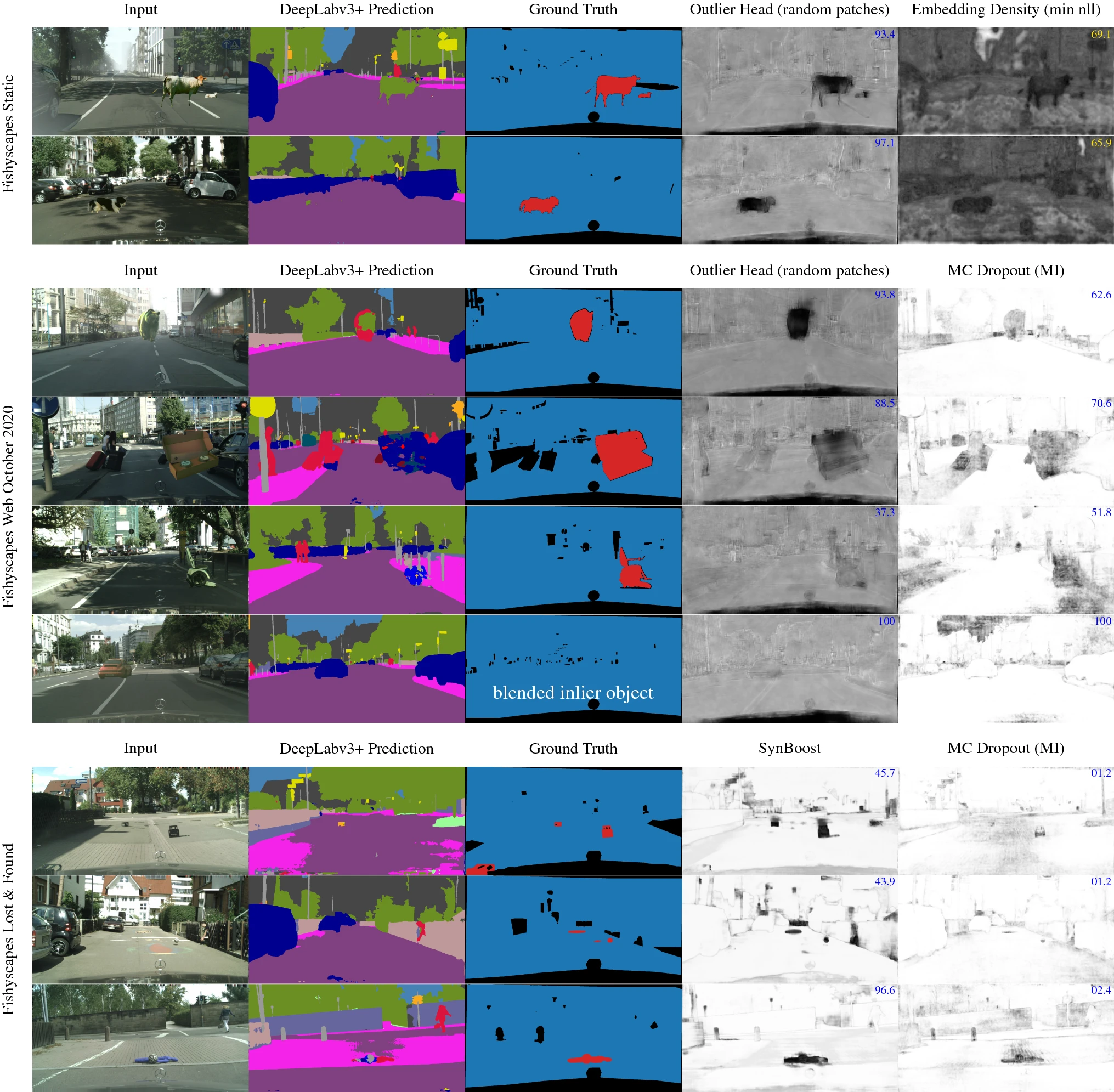
The following figure from the Fishyscapes paper shows some of the images from the datasets along with the ground truth masks and the outputs of some models. The Fishyscapes Static dataset and the Fishyscapes Web dataset contain synthetic images, while the Fishyscapes Lost & Found dataset contains real images.
The two main metrics used to evaluate methods are Average Precision (AP) and False Positive Rate at 95% True Positive Rate (FPR95). Average Precision is the mean precision over all possible recall values. FPR95 is also used since high true positive rates are important in safety-critical applications.
Deep Neighbor Proximity
Surprisingly, one of the top methods as measured by AP is based on a simple kNN approach described in [2], called Deep Neighbor Proximity (DNP). The basic idea is to take feature vectors from the hidden layers of a semantic segmentation model and compute the L2 distances from those vectors to a set of reference features computed using the same model on the training data. The average distance to the \(k\) nearest neighbors is used as the OoD score (\(k = 3\) was found to give the best results). The assumption is that OoD objects will have feature vectors that are further away from the reference feature vectors since they are not similar to anything in the training data, so the average distance to the \(k\) nearest neighbors will be higher.
Feature Selection
DNP can be applied to both CNN and transformer architectures. For CNNs, the output of one of the intermediate convolutional layers is used as the features. The feature vector of a pixel consists of the value of that pixel in each of the feature map’s channels. For transformer architectures, using the queries, keys, or values inside a block as features was found to be better than using the output of a block.
Combined Deep Neighbor Proximity
One naive way to detect anomalies is to measure how spread out the predictions of the semantic segmentation model are using operations like LogSumExp. The assumption is that OoD objects will result in predictions that are more spread out since the model will be less confident. This performs poorly on its own unless the model was specifically trained to output uniform distributions on OoD data, but it performs well when combined with DNP. Combined Deep Neighbor Proximity (cDNP) combines the scores from DNP and the LogSumExp of the predictions by rescaling them and adding them together.
Results
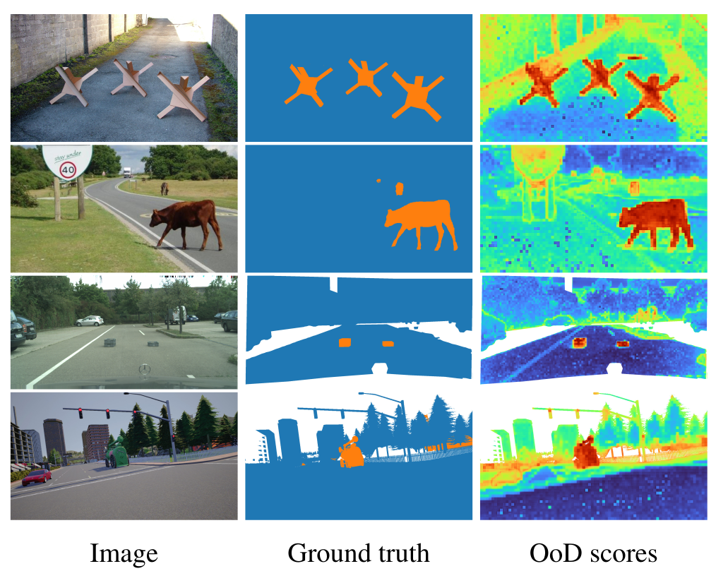
When applied to the Segmenter-ViT-B model [3], cDNP achieves an AP of 62.2% and a FPR95 of 8.9% on Fishyscapes Lost & Found. Here’s a figure from the paper that shows some of the OoD scores obtained using cDNP:
Advantages and Disadvantages
A major advantage of cDNP is that it does not require OoD data, which is difficult to obtain as explained previously. It can be applied to an existing segmentation model without modifying the model or doing any additional training, while some other methods can decrease the model’s segmentation accuracy.
The major disadvantage for kNN methods is the computational cost of finding the \(k\) nearest neighbors of every feature vector. The Fishyscapes leaderboard shows that cDNP is slower than many other methods.
NFlowJS
NFlowJS detects anomalies by training a segmentation model to maximize prediction entropy on synthetic OoD data [4]. The synthetic data is generated using a normalizing flow model, which is a sequence of learned bijective mappings that transform a Gaussian distribution to the generated image. The output of the normalizing flow is pasted into a random patch of a regular image from the segmentation dataset and used to train the segmentation model. The authors of the paper used Ladder DenseNet-121 [5] as the segmentation model and DenseFlow-25-6 [6] as the normalizing flow.
Training Process
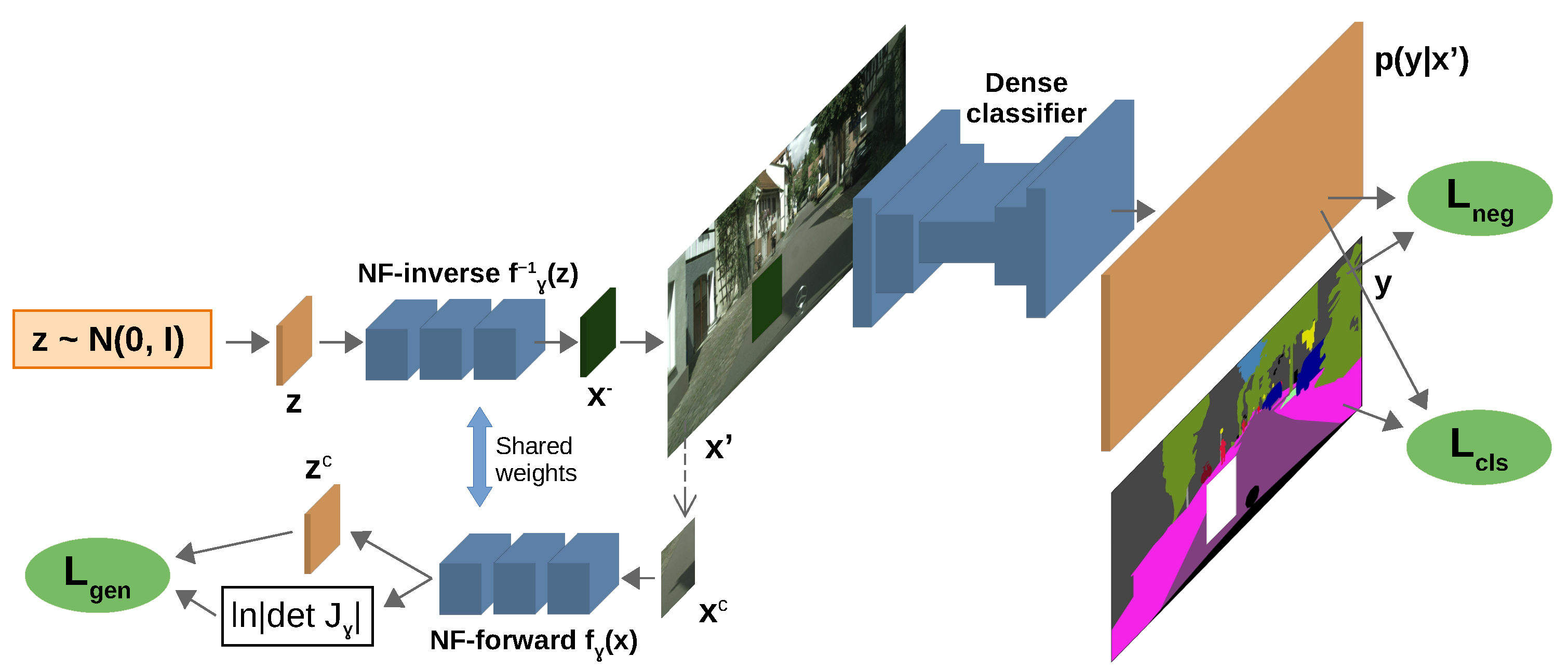
The segmentation model is trained to accurately classify the inlier pixels while outputting uniform predictions for the outlier pixels. The loss for inlier pixels is the regular cross-entropy loss, while the loss for outlier pixels is the JS divergence between the uniform distribution and the model’s predicted probabilities multiplied by a hyperparameter coefficient. These losses are added together to obtain the segmentation model’s loss, and the JS divergence is also used as the OoD score. The normalizing flow is trained to maximize the likelihood of the inlier patch from the dataset image that is replaced by the generated outlier patch, while also causing the segmentation model to output uniform predictions for the generated patch. The loss is the sum of the negative log-likelihood for the inlier patch and the segmentation model’s loss for the outlier pixels. The paper argues that this makes the normalizing flow generate patches that are on the edge of the distribution in the training set. In other words, the patches are somewhat similar to patches from the training images but are different enough to be classified as outliers. This figure from the paper illustrates the training process:
Results
NFlowJS achieved an AP of 69.43% and a FPR95 of 1.96% on Fishyscapes Lost & Found. The following image from the paper shows some of the patches generated by the normalizing flow:
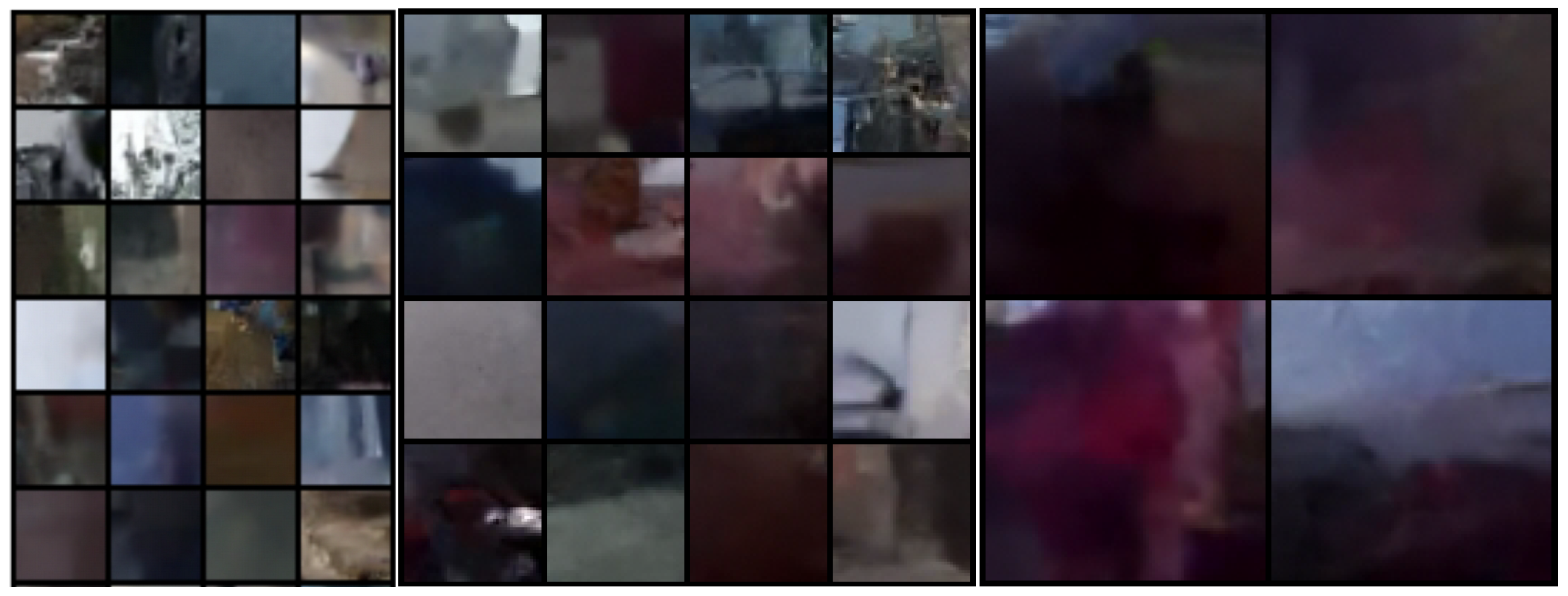
As expected, the patches vaguely resemble parts of the training images, but don’t look realistic.
Advantages and Disadvantages
NFlowJS retrains the model on data containing OoD objects, but it does not require an OoD dataset since it uses the normalizing flow to generate its own synthetic data. A disadvantage compared to cDNP is that retraining takes time and could impact the model’s segmentation performance. On the other hand, the inference speed should be close to the speed of the original segmentation model, since the only additional work at inference time is calculating the OoD scores from the model’s predictions.
References
[1] Blum, H., Sarlin, P.-E., Nieto, J., Siegwart, R., & Cadena, C. (2021). The Fishyscapes Benchmark: Measuring Blind Spots in Semantic Segmentation. International Journal of Computer Vision, 129(11), 3119–3135. https://doi.org/10.1007/s11263-021-01511-6
[2] Galesso, S., Argus, M., & Brox, T. (2023). Far Away in the Deep Space: Dense Nearest-Neighbor-Based Out-of-Distribution Detection. In 2023 IEEE/CVF International Conference on Computer Vision Workshops (ICCVW) (pp. 4479–4489). https://doi.org/10.1109/ICCVW60793.2023.00482
[3] Strudel, R., Garcia, R., Laptev, I., & Schmid, C. (2021). Segmenter: Transformer for Semantic Segmentation. In 2021 IEEE/CVF International Conference on Computer Vision (ICCV) (pp. 7242–7252). https://doi.org/10.1109/ICCV48922.2021.00717
[4] Grcić, M., Bevandić, P., Kalafatić, Z., & Šegvić, S. (2024). Dense Out-of-Distribution Detection by Robust Learning on Synthetic Negative Data. Sensors, 24(4), 1248. https://doi.org/10.3390/s24041248
[5] Krešo, I., Krapac, J., & Šegvić, S. (2021). Efficient Ladder-Style DenseNets for Semantic Segmentation of Large Images. IEEE Transactions on Intelligent Transportation Systems, 22(8), 4951–4961. https://doi.org/10.1109/TITS.2020.2984894
[6] Grcić, M., Grubišić, I., & Šegvić, S. (2021). Densely connected normalizing flows. In Advances in Neural Information Processing Systems (Vol. 34, pp. 23968–23982). Curran Associates, Inc. https://proceedings.neurips.cc/paper/2021/hash/c950cde9b3f83f41721788e3315a14a3-Abstract.html. Accessed 20 March 2024