Natural Image Classification
Natural image classification involves the process of developing and training machine learning models capable of accurately assigning labels to images depicting real-world objects, landscapes, and scenes at a scale decipherable to humans. In the project, we will cover traditional approaches as well as deep learning approaches to tackle this problem.
Introduction
Natural image classification involves the process of developing and training machine learning models capable of accurately assigning labels to images depicting real-world objects, landscapes, and scenes at a scale decipherable to humans. These images encompass a broad spectrum of subjects, including animals, buildings, trees, and various other entities encountered in everyday life. The task of classification entails training machine learning algorithms to recognize and categorize these diverse visual inputs into predefined classes or categories. This process not only serves as a fundamental component of computer vision but also finds applications across numerous domains, such as autonomous vehicles, medical imaging, and surveillance systems. Achieving robust classification performance demands the utilization of sophisticated deep learning architectures trained on vast datasets, enabling the model to generalize effectively across a wide range of classes and accurately classify unseen images.
Datasets
Numerous public datasets exist for natural images. Unlike certain domains such as medical imaging, natural images are significantly easier to gather and have less requirements in how the image has to be taken. ImageNet is perhaps the most famous dataset, with more than 14 million images and 20,000 categories. Often, ImageNet-1k is preferred due to computational limitations, which instead only has 1000 classes. Another popular dataset is CIFAR-10, and CIFAR-100, which contain 10 and 100 categories respectively. There also exist a variety of datasets for more specific subsets of natural images, such as cats vs dogs. Generally, for most tasks in natural image classification a sufficiently large dataset exists.
Traditional Methods
The advancement of image classification technology primarily stems from the field of machine learning. Classical methodologies revolve around leveraging training data to craft statistical models, thereby empowering computers with the capability to predict and analyze untrained data. A plethora of classification algorithms exist, ranging from foundational techniques like linear regression and decision trees (including random forests) to more sophisticated approaches such as neural networks, support vector machines, Bayesian classifiers, and clustering.
Deep Learning Methods
Compared to classical approaches, there are many advantages to using deep learning over these traditional methods. Classical approaches often rely on feature extraction methods, where humans design algorithms to identify relevant features in the data. However, these handcrafted features might not capture the full complexity of natural images. Deep learning, particularly Convolutional Neural Networks (CNNs), learns hierarchical representations of features directly from the raw pixel data. This allows the model to automatically discover and extract patterns and structures present in the images without the need for explicit feature engineering. Classical approaches typically have fixed feature extraction pipelines, making them less adaptable to different datasets or domains. They may struggle to generalize well across diverse image datasets. On the other hand, deep learning models are flexible and can adapt to various data distributions and complexities. They learn representations directly from the data, enabling them to generalize effectively to unseen images and different tasks with minimal manual intervention. Natural images often contain complex relationships and dependencies between pixels, such as spatial hierarchies of features and contextual information. Deep learning models, especially CNNs, are designed to capture these complex relationships through their hierarchical architecture. Each layer learns increasingly abstract features by aggregating information from previous layers, allowing the model to effectively encode the information present in natural images. As datasets grow larger and more diverse, scalability also becomes a crucial factor in image classification tasks. Deep learning frameworks, supported by GPUs, and TPUs, enable efficient training of large-scale models on massive datasets. This scalability empowers deep learning models to handle the increasing complexity and volume of image data effectively.
CNNs
Convolutional Neural Networks (CNNs) have been considered the state-of-the-art deep learning model for image tasks. Through a series of so-called convolution and pooling layers, they extract low-level features like edges and textures from the image in the initial layers, gradually transitioning to more abstract and complex features in deeper layers.
The core building blocks of CNNs, convolutional layers, apply filters (also known as kernels) to input images, extracting spatial patterns by performing convolutions. These filters are learned during the training process, allowing the network to adapt to the specific characteristics of the dataset. Convolutional layers enable CNNs to capture local patterns and spatial relationships, essential for recognizing objects within images.
Following convolutional layers, pooling layers downsample feature maps, reducing their spatial dimensions while retaining the most salient information. Common pooling operations include max pooling and average pooling, which help make the network more robust to variations in the input, improve computational efficiency, and enhance translation invariance.
Activation functions like ReLU (Rectified Linear Unit) introduce non-linearities into the network, enabling CNNs to model complex, non-linear relationships within the data. ReLU, in particular, has become the standard choice due to its simplicity and effectiveness in mitigating the vanishing gradient problem during training.
Towards the end of the network, fully connected layers combine the features extracted by convolutional and pooling layers to make predictions. These layers typically employ techniques like softmax activation to produce class probabilities, enabling the network to classify images into different categories.
Over the years, various architectural innovations have been proposed to improve CNNs’ performance and efficiency. This includes techniques like skip connections (e.g., in ResNet), attention mechanisms, and network pruning, which aim to address issues like vanishing gradients, capture long-range dependencies, and reduce model size and computational complexity. Hence, their ability to automatically learn discriminative features from raw pixel data makes them extremely useful for image classification.
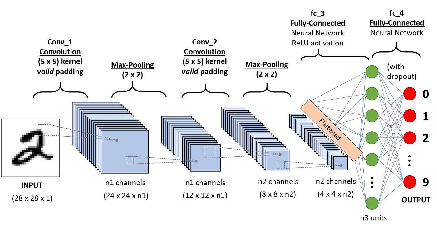
Fig 1. A simple convolutional neural network [1].
Resnets
One problem that limited the performance of CNN models was that at a certain point, increasing depth would actually decrease model performance. This was largely due to the issue of vanishing gradients, which meant that deeper models would have a hard time optimizing their highest layers to be able to properly detect features. In order to resolve this, ResNets learn a residual mapping by making use of a skip connection, as seen in Figure 2. This allows much deeper networks, e.g. Resnet-152 with 152 layers, to exist. This allows for the model to support more parameters and represent finer details, improving performance over traditional CNNs.
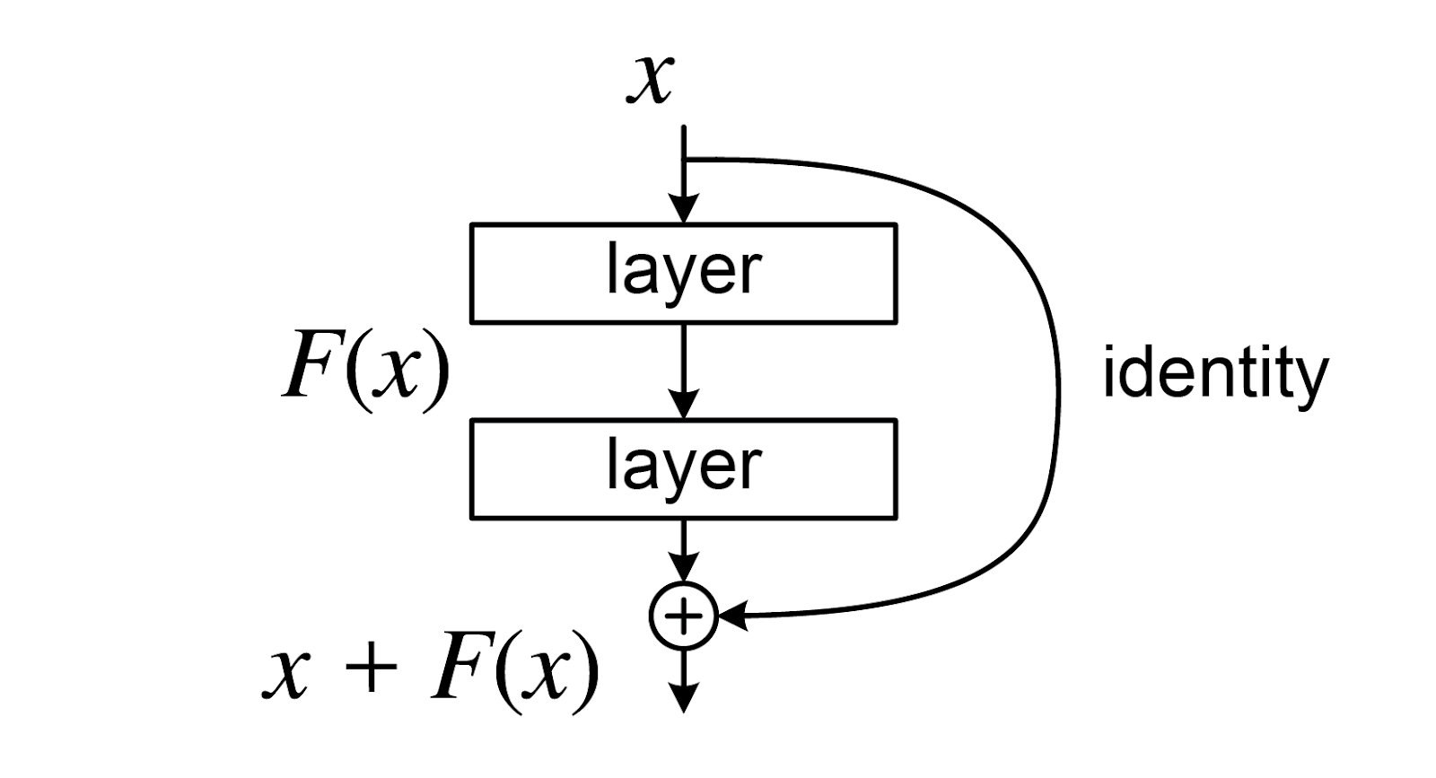
Fig 2. Skip connection [2].
Vision Transformers
Transformers are a somewhat new type of model that were originally created for natural language processing, but have been extended to be used for computer vision tasks as well. The original transformer includes 2 parts, an encoder and a decoder. Vision Transformers only include the encoder portion.
Vision Transformers take an image and split it up into patches, which then gets fed through the encoder. Inside the encoder, patches are turned into an embedding and are combined with their positional encoding, which makes use of the spatial location of each patch. The encoder applies self-attention on these embeddings, which gets an output that gives relation about each pair of input. Afterwards, we add the original input (a residual connection, the same as in ResNets) and normalize, before sending them through a multi-layer perceptron that gives the output. This output is also added with the input before the feed-forward network (residual connection again) and normalized. For Vision Transformers, this encoder output is then fed through another multi-layer perceptron to get the class scores.
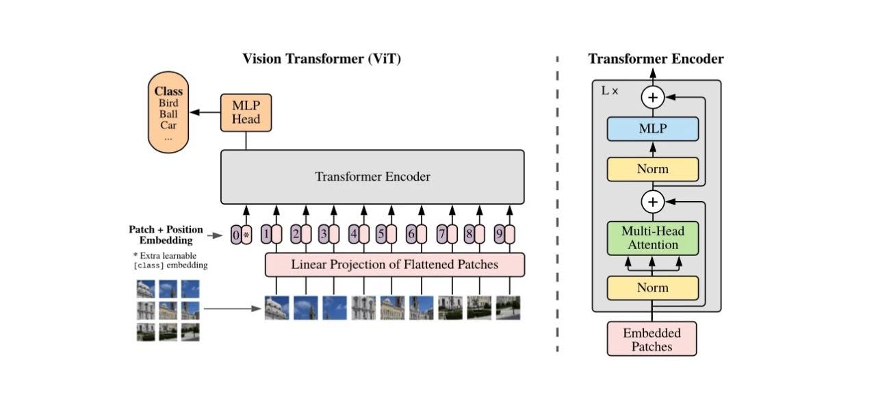
Fig 3. The Vision Transformer Architecture [3].
CoAtNet
Although Vision Transformers empirically outperform CNN models, this is only when the Vision Transformer is trained for a long time, and typically on datasets with tens or hundreds of millions of images. When trained on smaller datasets, CNNs typically outperform Vision Transformers. This hints that CNNs might have some beneficial inductive bias that Vision Transformers lack. CoAtNet is a family of models that aims to combine the two in a way that performs either model type individually. On ImageNet, the paper’s best CoAtNet model was able to achieve a 90.88% top-1 accuracy, which is state-of-the-art.
One of the building blocks of CoAtNets is the MBConv block, which is a convolutional block that makes use of depthwise convolution layers. In depthwise convolution, filters are convolved over input features channel-wise (i.e. one channel at a time), rather than over all channels and have one filter for each channel. This reduces the amount of parameters needed for a convolutional block greatly.
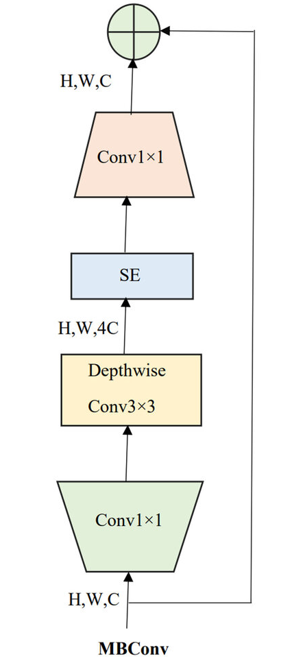
Fig 4. MBConv Block [4].
CoAtNets also use relative attention, rather than the absolute self-attention in traditional Transformers. This is one of the two main ways they combine CNNs and transformers. By taking a look at the mathematical representation for depthwise convolution and the original absolute self-attention, the authors were able to combine the two into the shown relative attention formula. This is nice as depthwise convolution captures the relative position and maintains translational equivariance (which has empirically improved model generalization under a limited dataset), while the original self-attention portion still captures the pairwise relationship between out inputs. This also maintains the global receptive field in the origin self-attention.
Depthwise Convolution:
\[y_i = \sum_{\substack{j \in \mathcal{L}(i)}} w_{i-j} \odot x_j\]Original Self-Attention:
\[y_i = \sum_{j \in \mathcal{G}} \frac{\exp(x_i^T x_j)}{\sum_{k \in \mathcal{G}} \exp(x_i^T x_k)} x_j\]Combined Relative Attention:
\[y_i^{pre} = \sum_{j \in \mathcal{G}} \frac{\exp(x_i^T x_j + w_{i-j})}{\sum_{k \in \mathcal{G}} \exp(x_i^T x_k + w_{i-k})} \cdot x_j\]The second way they combined the two is in the model architecture itself, which features 2 sets of convolution blocks before 2 sets of relative-attention blocks. The model first starts with a stem stage, which downsamples the image size, and also downsamples the image before each convolution block and each relative-attention block. As shown, the network also makes use of residual connections, the same as in ResNets.
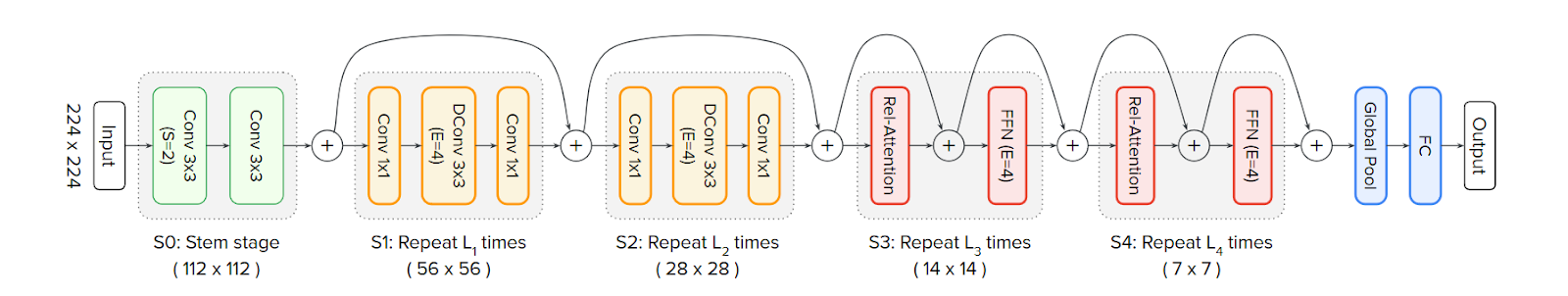
Fig 5. CoAtNet Model Architecture [4].
Experiments and Results
We compared the performance between a ResNet and Vision Transformer. Due to limited compute resources and time, we train on only 3 epochs for all models, and we train the models from scratch rather than using pre-trained weights. The models were trained and evaluated on the Imagenet dataset, which has only 10 classes and is a much smaller subset of the ImageNet dataset. We use Hugging Face to load and train the models. Specifically, we use ResNet-50 and ViT-base. Below is the code for the initialization of those models.
configuration = ResNetConfig(
    num_labels=10,
    label2id=label2id,
    id2label=id2label,
    ignore_mismatched_sizes = True)
model = ResNetForImageClassification(configuration)

configuration = ViTConfig(
    num_labels=10,
    label2id=label2id,
    id2label=id2label,
    ignore_mismatched_sizes = True)
model = ViTForImageClassification(configuration).to(device)
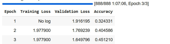
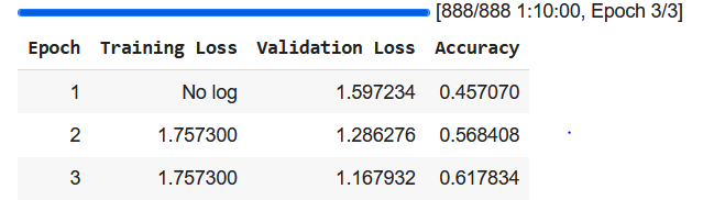
Below you can see the results for both. For this dataset, ViT-base performed much better than ResNet-50. Although empirically it has been shown that CNNs often perform better than ViTs on smaller datasets, it’s likely that relatively simple ResNet-50 is too lacking compared to newer state-of-the-art CNNs that apply more advanced mechanisms and have deeper layers. The ResNet achieved an accuracy of 45% on our validation dataset while the ViT achieved an accuracy of 62% after 3 epochs.
ResNet results
ViT results
Code
The full code for the experiments can be found here Full Notebook
References
[1] Ratan, Phani “What is the Convolutional Neural Network” https://www.analyticsvidhya.com/blog/2020/10/what-is-the-convolutional-neural-network-architecture/ 2023.
[2] He, Kaiming, et al. “Deep Resiudal Learning for Image Recognition.” arXiv preprint arXiv:1512.03385v1 2015.
[3] Dosovitskiy Alexey, et al. “An Image is Worth 16x16 Words: Transformers For Image Recognition At Scale.” arXiv preprint arXiv:2010.11929v2 2021.
[4] Dai, Zihang, et al. “CoAtNet: Marrying Convolution and Attention for All Data Sizes.” arXiv preprint arXiv:2106.04803v2 2021.