Fine-tuning Stable Diffusion with Dreambooth
Stable diffusion is an extremely powerful text-to-image model, however it struggles with generating images of specific subjects. We decided to address this by exploring the state-of-the-art fine-tuning method DreamBooth to evaluate its ability to create images with custom faces, as well as its ability to replicate custom environments.
- Introduction
- How Diffusion Works
- Diffusion: Forward Process
- Diffusion: Reverse Process
- Stable Diffusion
- Autoencoders
- VAEs
- UNet Backbones
- Text conditioning / CLIPTokenizer
- Stable Diffusion XL
- DreamBooth Internal
- Pipeline
- Novel Implementation
- Training Script
- Results
- Conclusion
- Reference
Introduction
We address the limitations of stable diffusion models in generating images of specific subjects and environments by applying a state-of-the-art fine-tuning method known as DreamBooth, which enables the model to recognize and generate specific subjects or styles. We proceed with two main objectives: to assess DreamBooth’s effectiveness in creating images with faces, and to evaluate its capability in accurately replicating custom environments across multiple diffusions – a novel exploration since DreamBooth has predominantly focused on replicating specific objects. We conducted experiments using datasets specifically curated for these tasks, fine-tuning the Stable Diffusion and Stable Diffusion XL models in conjunction with DreamBooth. The results demonstrate a significant improvement in the model’s ability to produce detailed and contextually appropriate images, showcasing DreamBooth’s potential in enhancing the specificity and relevance of generated images. This research contributes to the field of generative artificial intelligence by providing insights into methods for personalizing text-to-image models, with implications for advancing content creation in various creative industries.
How Diffusion Works
Diffusion is a generative technique that can be used to create images by gradually transforming a distribution of random noise into a coherent image using a deep neural network [1]. The process can be thought of as “denoising” and is based on the principles of diffusion processes observable in physical and biological systems.
Diffusion: Forward Process
The model is first trained by applying a diffusion process to an image, which adds Gaussian noise to the image over many steps (1,000 or so) until the image is complete noise. When adding Gaussian noise to an image, what is essentially occurring is the pixel values of the image are being modified by adding a small (or large, depending on the variance) random amount to each pixel. The randomness is guided by the Gaussian or Normal distribution, meaning most pixel changes will be small – close to the mean – but a few might be larger. Thus, the difference from Step i to Step i+1 is small, but over the 1,000 steps, the image becomes pure noise.
Diffusion: Reverse Process
The reverse process is where the actual learning and image creation take place. Essentially, the model iteratively predicts and removes the noise added during the forward process, attempting to reconstruct the original input image. The process begins with a sample of pure noise, with no recognizable structure or content related to the desired output image. At each step, the model, which has been trained on many examples of partially noised images and their corresponding noise patterns, tries to predict the exact noise that was added to the image at the corresponding step of the forward process. The model therefore makes an educated guess about how much of the current image’s content is noise versus signal (the underlying image structure). Once the model makes its prediction about the noise, this predicted noise is subtracted from the current image. This step is denoising, where the model effectively reverses one step of the forward process through removing the estimated noise. This process is repeated iteratively, as the model works its way back through the noise levels added during the forward process. With each step, the image becomes less noisy and more structured, gradually revealing the content and structure that the model has learned to generate. In conditional diffusion models, used for text-to-image generation, the denoising process is also conditioned on text descriptions, guiding the denoising to ensure the output image aligns with the given condition. The final output of the reverse process is a fully-denoised image, with a structure and clear image that was not apparent in the pure noise sample. The model is trained by exposing it to many examples of images at various stages of the forward (noising) process, alongside exactly how much noise was added at each step. Thus, the model learns the characteristics of the noise and how to properly remove it.
Stable Diffusion
Stable Diffusion is an important step forward for diffusion models. It was published to be a more robust, lightweight, accessible form of diffusion. The main change was performing the noising/denoising process in the latent space, as opposed to the image space [2]. In the following sections we will detail the variational autoencoders, backbones, and tokenizers used to facilitate this latent diffusion process. It is built to be open source, accessible, and easy to use on consumer grade graphics cards. Downloading the pretrained model allows you to generate images in a matter of minutes, while maintaining control over hyperparameters. The lightweight model works because image features are preserved in the latent space, and fine details can be painted in post-diffusion by variational autoencoders.
Autoencoders
Autoencoders are key to the process of dimensionality reduction in stable diffusion. By compressing data into the latent space, and reducing the number of features describing the input, it lets our diffusion model easily manipulate, select, and extract information from the original dataset. Comprised of an encoder and a decoder, the autoencoder compresses a 512x512 pixel image down to a 64x64 model in the latent, where diffusion is performed, before the decoder reconstructs a pixel image of the same size as the input. This process typically results in data loss during the decoding process. Our aim for an efficient autoencoder model is to optimize the encoder/decoder pair to preserve maximal information during compression, and to decode with minimal information loss. We can calculate loss on the AE by observing the difference between an input image \(x\) and the image \(\bar{x}\) which is the pixel image created by running the encoder on \(x\) and then the decoder on the resulting latent model. The loss function to represent this is as follows \(|x - \bar{x}|_2 = |x - d(e(x))|_2\). This loss is used for gradient descent and backpropagation to optimize the autoencoder.
VAEs
Variational autoencoders (VAEs) improve on standard autoencoders by introducing probabilistic modeling into the encoding process. VAEs use neural network architectures for unsupervised learning of a probabilistic distribution in the latent space. This enables more effective sampling and interpolation between data points. VAEs can generate more diverse and realistic outputs than traditional autoencoders, while also providing a structured and continuous latent space representation. Additionally, they offer a more robust framework for regularization and control over the latent space, facilitating better disentanglement of underlying factors in the data. In general, VAEs provide a more versatile and powerful framework for tasks such as image generation, data generation, and representation learning.
UNet Backbones
UNet backbones are the most commonly used backbone architectures, and they are crucial to the diffusion process. UNets, also aptly called Noise Predictors, provide the essential ability to predict the amount of noise in an image \(x_t\), given that image and its corresponding time step \(t\). This information is used during denoising in the reverse pass of stable diffusion. The UNet is a convolutional neural network that consists of downsampling followed by upsampling, with a series of long skip connects (LSCs) as shown in the image.
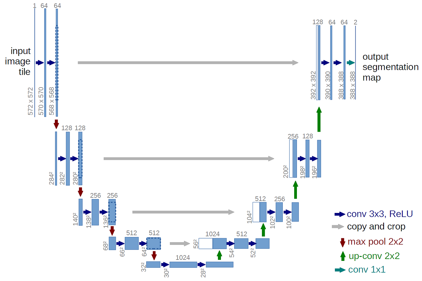
This structure optimizes a few things. First the downsampling/upsampling process fuses image features together to form a denser, more informative feature map. The LSCs help the model to aggregate long distance information, and address the vanishing gradient problem. The UNet backbone can now recognize both local and global features effectively, and does a good job of preserving spatial information. They are computationally efficient, and robust to variations in the input. All of these advantages make the UNet architecture the premier noise predictor in diffusion models.
Text conditioning / CLIPTokenizer
For a text-to-image generative model like the one we are implementing, we must condition the model based on the input text. The tokenizer aims to construct a model input of up to 75 unique tokens from the given text. Each word the tokenizer reads is wrapped into a 768-value vector token, containing embedded data about the input. The CLIP model is pre-trained on SOTA image captioning datasets, so it can be called efficiently within stable diffusion models. Newer CLIP models analyze subsections of the input text instead of a single word at a time, taking the context of each word into account allows these tokenizers to perform better in testing. The output tokens are passed as an input to the UNet backbone in order to perform noise prediction.
Stable Diffusion XL
Recently, Stability AI published an even more powerful stable diffusion model called Stable Diffusion XL (SDXL). SDXL improves on many parts of stable diffusion, most noticeable in its capabilities to generate highly photorealistic, finer quality images [3]. It requires significantly more compute power than the older models, with over 3.5 billion learnable parameters (3x more than any prior stable diffusion model). This model takes in 1024x1024 px images, has a larger UNet backbone, and operates in a larger latent space. All of this allows SDXL to cover a wider range of visual styles, along with generating more accurate faces, hands, and legible text. These fine grained capabilities are appealing to many fields in CV, thus the heavier model has become popular, even amongst longer training times and more required computation.
DreamBooth Internal
In addressing the nuances of few-shot learning, the focus is on refining text-to-image diffusion models to prevent overfitting and retain a diverse knowledge base. To overcome these bottlenecks, the author proposed a new loss function, Class-specific Prior Preservation Loss to supervise the model more effectively [4].
Reconstruction Loss
To understand the new method the author proposed, we need to understand how the original loss function works for diffusion models:
\[\mathbb E_{x, c, \epsilon, t}[w_t || \hat x_\theta (\alpha _t x + \sigma_t\epsilon, c) - x ||^2_2]\]where \(x\) is the ground-truth image, \(x_{\theta}\) is the output image, \(c\) is a conditioning vector, which is a text prompt in this case. \(\epsilon\) is the noise we add to the image with normal distribution. \(\alpha_t, \sigma_t, w_t\) are terms for noise scheduling and sample quality, with time step \(t\).
Rare Unique Identifier Token
The author introduced a new approach by implanting a new unique identifier token into the model’s “dictionary”, with a format of: “a [identifier] [class noun]”, where [identifier] is a unique identifier linked to the subject and [class noun] is the class that you want to associate with.
Autogenous Class-specific Prior Preservation Loss
Now we can add the prior-preservation term to the previous loss. It becomes
\[\mathbb E_{x, c, \epsilon, t}[w_t || \hat x_\theta (\alpha _t x + \sigma_t\epsilon, c) - x ||^2_2 + \lambda w_t'||\hat x_\theta (\alpha' _t x_{pr} + \sigma_t'\epsilon', c_{pr}) - x_{pr} ||^2_2]\]where \(x_{pr}\) is the image generated by the frozen model, \(c_{pr}\) is the text prompt without the rare token. \(\lambda\) is used to give the second term a weight, and the author set it to one.
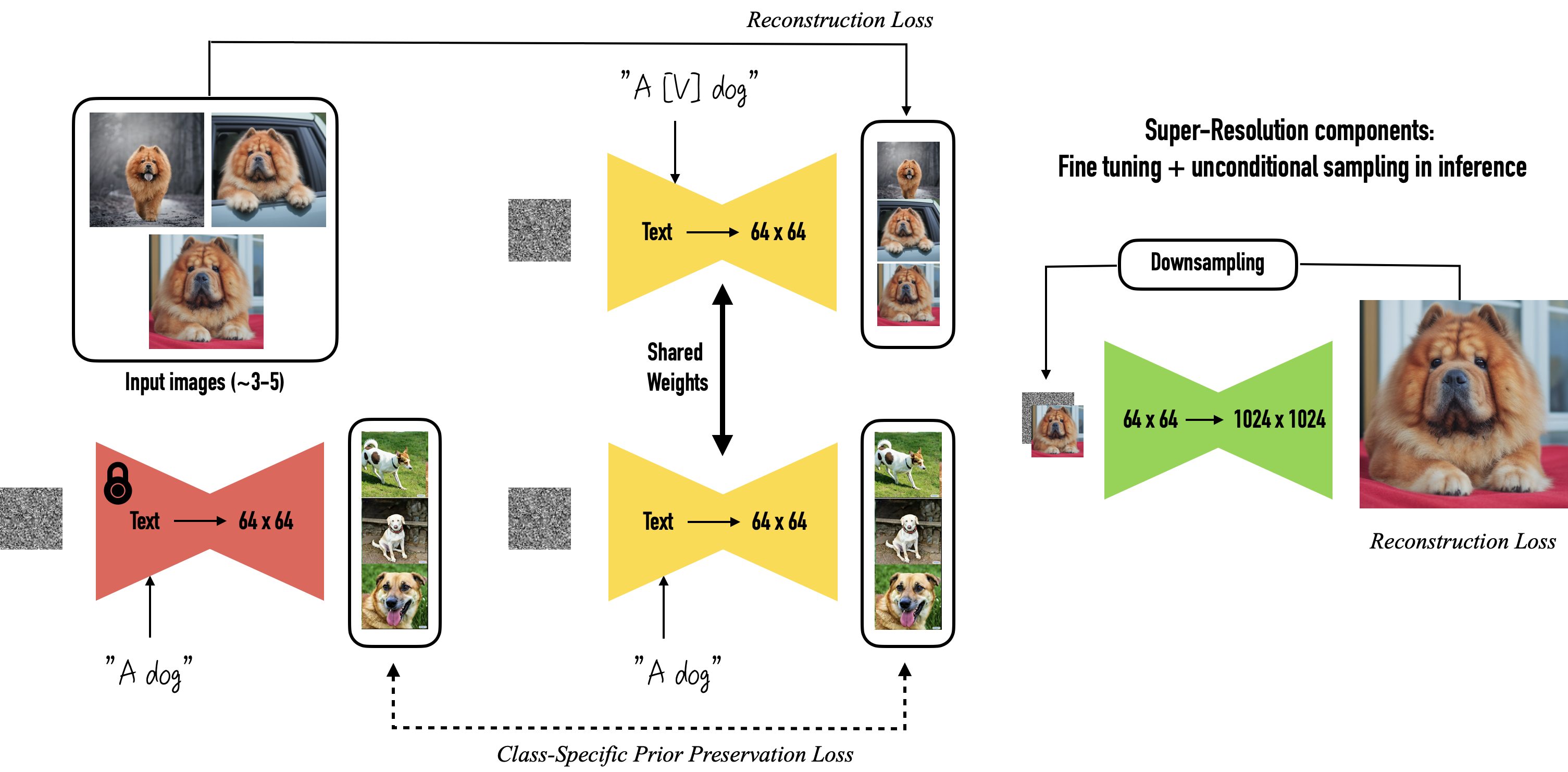
Pipeline
With the new loss function and the unique identifier, we can start fine tuning the model. Firstly, we give the model the specific type of image that we want the model to fine-tune on as input, then prompt the (yellow) model with the format mentioned above including the rare token to train it. This part is to link the model with the type of image we want, and it’s supervised by the reconstruction loss.
Secondly, we take an off-the-shelf text to image model(the red one) to generate images with the usual text prompt “a [class noun]”. Compare the output of the red model with the yellow one. This part ensures the new model is grounded with the existing knowledge with the class. Combined with the first part, we supervise this task with the autogenous class-specific prior preservation loss.
The integration of the autogenous class-specific prior preservation loss and the unique identifier in the fine-tuning process significantly enhances few-shot image generation. This method not only ensures detailed and accurate image generation but also safeguards the model’s ability to produce diverse instances within a given class, maintaining a delicate balance between specificity and generality.
Novel Implementation
DreamBooth allows saving of a specific object across multiple diffusions, in different environments. A novel approach explored was saving a specific environment across multiple diffusions, with different objects. In effect, instead of an object being the constant, now the environment is the constant.
To proceed, we fine-tuned both Stable DIffusion and Stable Diffusion XL and compared the results. Importantly, we fine-tuned using LoRA (Low-Rank Adaptation), which offers a powerful approach to personalizing large-scale generative models for specific styles, while still maintaining the efficiency and generality of the original model. LoRA implements low-rank matrices, much smaller than the original model’s weight matrices, that capture the essence of the necessary adaptation without significantly altering the entire model. Therefore, LoRA is able to finetune the model without adjusting all original weights. In particular, LoRA has fewer trainable parameters during fine-tuning, making it more memory efficient and causing the forward and backward passes to be computed more efficiently.
Training Script
Now that you have an idea of how the DreamBooth training method works, let’s dive into an example of how it is utilized in practice.
The de-facto standard for anything related to diffusion is the python library diffusers created by Hugging Face. It provides primitives and pretrained diffusion models for use across several domains like image and audio generation.
In this case we used their train_dreambooth script in combination with their pretrained Stable Diffusion and SDXL models to run our experiments.
Script overview
To finetune raw Stable Diffusion, we ran the script with the following command which reveals our chosen hyper parameters:
accelerate launch ./diffusers/examples/dreambooth/train_dreambooth.py \
  --pretrained_model_name_or_path="runwayml/stable-diffusion-v1-5" \
  --instance_data_dir="./train_data" \
  --output_dir="finetuned_model" \
  --instance_prompt="A photo of rory" \
  --resolution=512 \
  --train_batch_size=1 \
  --gradient_accumulation_steps=1 \
  --learning_rate=5e-6 \
  --lr_scheduler="constant" \
  --lr_warmup_steps=0 \
  --max_train_steps=400 \
  --train_text_encode
As you can see, we load the pretrained Stable Diffusion model, provide our training data and a label for each image. Additionally, we train for 400 steps with a constant learning rate of 5e-6. Another thing to note is that we instruct the script to retrain the text encoder with the flag --train_text_encode. We found this to be incredibly important for image quality, particularly in generating images of faces. This makes sense as it helps the model distinguish between text encodings for the provided training faces and its preconceived notion of a face.
Using this script, 6 training images and an A100 GPU, we were able to train the model in around 4 minutes.
Let’s take a closer look at the DreamBooth training script to see how it works under the hood. This script is from the diffusers library under the directory examples/dreambooth/train_dreambooth.py Considering that the actual training loop is around 400 lines of code, we have annotated the code and omitted many of the details for the sake of brevity. While not identical, the following code closely resembles the training loop in the script by highlighting the parts relevant to us.
for epoch in range(first_epoch, args.num_train_epochs):
    unet.train()
    text_encoder.train()
    for step, batch in enumerate(train_dataloader):
        pixel_values = batch["pixel_values"].to(dtype=weight_dtype)

        # Encode images into the latent space using provided vae
        if vae is not None:
            model_input = vae.encode(batch["pixel_values"].to(dtype=weight_dtype)).latent_dist.sample()
            model_input = model_input * vae.config.scaling_factor

        # Sample noise to add to the image
        noise = torch.randn_like(model_input) + 0.1 * torch.randn(
            model_input.shape[0], model_input.shape[1], 1, 1, device=model_input.device
        )

        # Sample a random timestep for each image
        timesteps = torch.randint(
            0, noise_scheduler.config.num_train_timesteps, (bsz,), device=model_input.device
        ).long()

        # Add noise to each image (forward diffusion)
        noisy_model_input = noise_scheduler.add_noise(model_input, noise, timesteps)

        # Create text embedding for conditioning using provided training label
        encoder_hidden_states = encode_prompt(
            text_encoder,
            batch["input_ids"],
            batch["attention_mask"],
            text_encoder_use_attention_mask=args.text_encoder_use_attention_mask,
        )

        # Add concatenate copy of noise to compute prior
        if unwrap_model(unet).config.in_channels == channels * 2:
            noisy_model_input = torch.cat([noisy_model_input, noisy_model_input], dim=1)

        # Predict noise residual
        model_pred = unet(
            noisy_model_input, timesteps, encoder_hidden_states, class_labels=class_labels, return_dict=False
        )[0]

        # Prior Preservation Loss
        target = noise
        if args.with_prior_preservation:
            # Chunk the noise and model_pred into two parts and compute the loss on each part separately.
            model_pred, model_pred_prior = torch.chunk(model_pred, 2, dim=0)
            target, target_prior = torch.chunk(target, 2, dim=0)
            # Compute prior loss
            prior_loss = F.mse_loss(model_pred_prior.float(), target_prior.float(), reduction="mean")

        # Compute Instance Reconstruction loss
        loss = F.mse_loss(model_pred.float(), target.float(), reduction="mean")

        if args.with_prior_preservation:
            # Add the prior loss to the instance loss.
            loss = loss + args.prior_loss_weight * prior_loss

        # Update parameters
        accelerator.backward(loss)
        if accelerator.sync_gradients:
            params_to_clip = (
                itertools.chain(unet.parameters(), text_encoder.parameters())
                if args.train_text_encoder
                else unet.parameters()
            )
            accelerator.clip_grad_norm_(params_to_clip, args.max_grad_norm)
        optimizer.step()

        # Adjust learning rate
        lr_scheduler.step()
        optimizer.zero_grad(set_to_none=args.set_grads_to_none)
Within this training loop we can see all of the main parts of Stable Diffusion as well as how they are integrated with DreamBooth.
First it loads a batch of images from the training dataset. This dataset includes all of the images provided for finetuning, and the standard batch size is 1 given the limited number of images.
# Load pixel values from batch
pixel_values = batch["pixel_values"].to(dtype=weight_dtype)

# Encode images into the latent space using provided vae
if vae is not None:
    model_input = vae.encode(batch["pixel_values"].to(dtype=weight_dtype)).latent_dist.sample()
    model_input = model_input * vae.config.scaling_factor
For each of these images, it samples Gaussian noise and adds it to the images in the batch at a random timestep according to the noise schedule.
# Sample noise to add to the image
noise = torch.randn_like(model_input) + 0.1 * torch.randn(
    model_input.shape[0], model_input.shape[1], 1, 1, device=model_input.device
)

# Sample a random timestep for each image
timesteps = torch.randint(
    0, noise_scheduler.config.num_train_timesteps, (bsz,), device=model_input.device
).long()

# Add noise to each image (forward diffusion)
noisy_model_input = noise_scheduler.add_noise(model_input, noise, timesteps)
Next it creates a text encoding for the prompt associated with the training image. This encoding will be used to condition the noise prediction U-net to associate our training images with the given prompt.
# Create text embedding for conditioning using provided training label
encoder_hidden_states = encode_prompt(
    text_encoder,
    batch["input_ids"],
    batch["attention_mask"],
    text_encoder_use_attention_mask=args.text_encoder_use_attention_mask,
)
Importantly, after this it concatenates a copy of the noise image which will allow for creation of a prior used to calculate the prior preservation loss later on.
# Add concatenate copy of noise to compute prior
if unwrap_model(unet).config.in_channels == channels * 2:
    noisy_model_input = torch.cat([noisy_model_input, noisy_model_input], dim=1)
Next, the model predicts the added noise using the pretrained U-net.
# Predict noise residual
model_pred = unet(
    noisy_model_input, timesteps, encoder_hidden_states, class_labels=class_labels, return_dict=False
)[0]
Up until this points, these steps have been similar to raw Stable Diffusion, however where Dreambooth is unique is in how it calculates the losses. First it calculates the prior preservation loss to measure deviation from the model’s preconceived notions of the input prompt.
 # Prior Preservation Loss
target = noise
if args.with_prior_preservation:
    # Chunk the noise and model_pred into two parts and compute the loss on each part separately.
    model_pred, model_pred_prior = torch.chunk(model_pred, 2, dim=0)
    target, target_prior = torch.chunk(target, 2, dim=0)
    # Compute prior loss
    prior_loss = F.mse_loss(model_pred_prior.float(), target_prior.float(), reduction="mean")
Next, the model computes the reconstruction loss and combines it with the weighted prior preservation loss.
# Compute Instance Reconstruction loss
loss = F.mse_loss(model_pred.float(), target.float(), reduction="mean")

if args.with_prior_preservation:
    # Add the prior loss to the instance loss.
    loss = loss + args.prior_loss_weight * prior_loss
As you can see, both of these losses are simply computed using mean squared error between the predictions and the ground truth.
Finally, it simply updates its weights and learning rate schedules.
# Update parameters
accelerator.backward(loss)
if accelerator.sync_gradients:
    params_to_clip = (
        itertools.chain(unet.parameters(), text_encoder.parameters())
        if args.train_text_encoder
        else unet.parameters()
    )
    accelerator.clip_grad_norm_(params_to_clip, args.max_grad_norm)
optimizer.step()

# Adjust learning rate
lr_scheduler.step()
optimizer.zero_grad(set_to_none=args.set_grads_to_none)
For more details on how we setup the environment to run these scripts, refer to our Fine Tuning Notebook.
Results
Overall we attempted to generate custom images using DreamBooth to fine-tune both Stable Diffusion and Stable Diffusion XL. These experiments included generating images of our faces and scenes from movies given the following training datasets:
- Dataset 1: A face from same perspective in same environment (6 images)
- Dataset 2: Frames from Blade Runner 2049 (5 images)
The purpose of having these different datasets was to evaluate the model’s capability to replicate custom objects and different environments.
Training images
Below are the images from each of the datasets along with our associated labels.
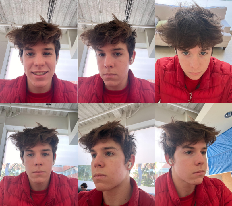 “A picture of Rory’s face”
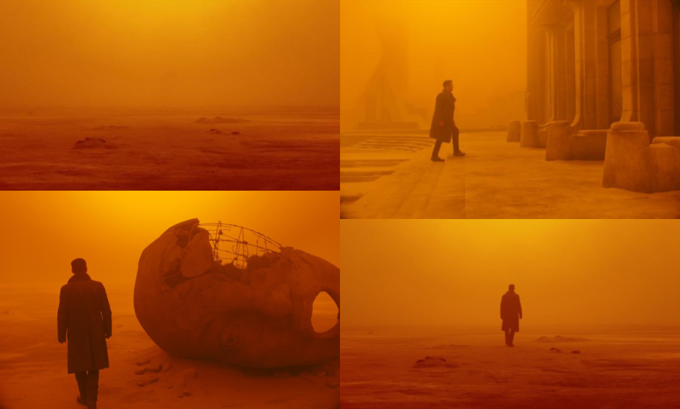 “A scene from the movie Blade Runner”
Stable Diffusion
Here are the results for creating custom face images using the following prompts.
- “A photo of Rory in the desert”
- “A photo of Rory holding a trophy in times square”
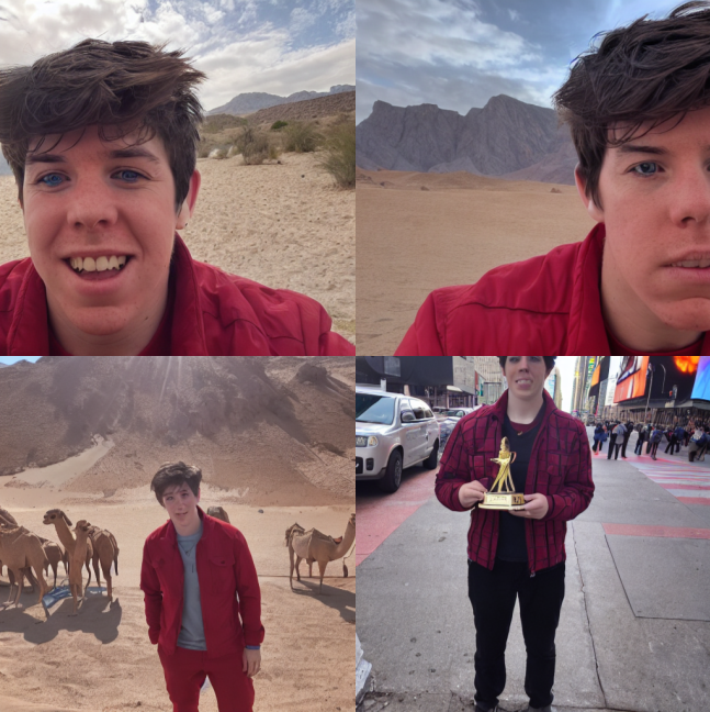 Images of custom faces generated using Finetuned Stable Diffusion
Here are the results from fine-tuning Stable Diffusion along with the Blade Runner images.
- “A dog walking in a scene from Blade Runner”
- “A car in a scene from Blade Runner”
- “The mona lisa in a scene from Blade Runner”
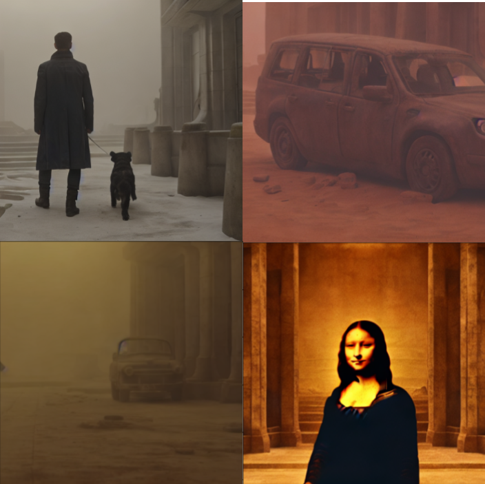 Images of custom Blade Runner scene generated using Finetuned Stable Diffusion
Overall, the results were good, but it’s clear that the model had some difficulty understanding the details of Rory’s face. However, it was astonishingly good at replicating the style and environment from just 4 images from one scene of a movie. While we knew that DreamBooth could replicate objects, the original authors never tested it on environments. According to these results, it clearly is capable of both.
Stable Diffusion XL
While the results from Stable Diffusion were pretty good, we wanted to experiment with Stable Diffusion XL to see if it would produce better quality images. Since Stable Diffusion XL is much larger, we expected better results, which turned out to be the case.
While using a slightly different script to fine-tune Stable Diffusion XL, we ended up using similar hyperparameters, except with a more aggressive learning rate of 1e-4 and 500 training steps. Something to note here is that we ended up using LoRA which allows us to save ram. This is particularly important as it significantly reduced training times and RAM usage, a critical step for SDXL because it is such a large model. Another thing to note is that we provide a third-part VAE model, as the stock Stability AI one is known to be flakey. Given its unwieldy size, it ended up taking around 1 hour to train using a V100 GPU and the following command:
# Stable Diffusion XL with LoRA
!accelerate launch diffusers/examples/dreambooth/train_dreambooth_lora_sdxl.py \
  --pretrained_model_name_or_path="stabilityai/stable-diffusion-xl-base-1.0" \
  --instance_data_dir="./train_data" \
  --pretrained_vae_model_name_or_path="madebyollin/sdxl-vae-fp16-fix" \
  --output_dir="finetuned_model_xl" \
  --mixed_precision="fp16" \
  --instance_prompt="A scene from star wars" \
  --resolution=1024 \
  --train_batch_size=1 \
  --gradient_accumulation_steps=4 \
  --learning_rate=1e-4 \
  --lr_scheduler="constant" \
  --lr_warmup_steps=0 \
  --max_train_steps=500 \
  --seed="0" \
  --enable_xformers_memory_efficient_attention \
  --gradient_checkpointing \
  --use_8bit_adam
Here are the results using the same prompts as before along with the following additional prompts.
- Rory Fighting a dragon
- A drawing of Rory’s face done in pencil
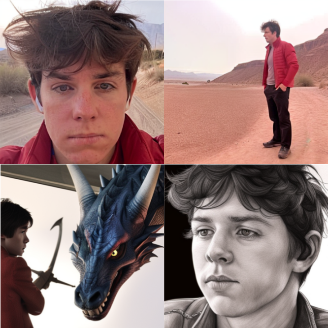 Images with Rory’s face generated using SDXL
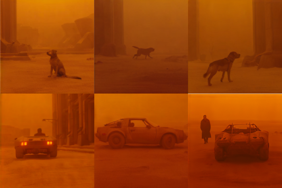 Blade Runner Images generated using SDXL
For SDXL, we also decided to train on a movie from an additional scene given how good the results were from Blade Runner. For this we used the following images from Star Wars in order to train.
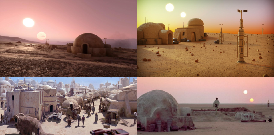 Training images used for Star Wars environment
Given these training images, here are the results on the following prompts:
- A car on Tatooine
- A dog on Tatooine
Here are the results:
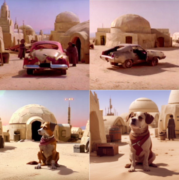 Images on Tatooine generated using SDXL
Overall, the SDXL results were amazing. It clearly outperformed Stable Diffusion with much higher quality images. Additionally, it seemed to have a much better understanding of faces given that it was able to reproduce the training face in different orientations and styles. It also had a deep understanding of the style established in the Blade Runner scene. It was even able to infer that the scene was set in the future by putting a futuristic looking car in the images without any sort of direction provided in the prompt or training images.
Conclusion
In conclusion, our exploration into DreamBooth’s application on stable diffusion models, specifically Stable Diffusion and Stable Diffusion XL, marks a significant stride towards addressing the challenge of generating highly specific and contextually relevant images. Through fine-tuning with DreamBooth, we have enhanced the models’ abilities to create precise representations of faces and environments, showcasing the potential for more personalized and accurate image generation within the field of generative artificial intelligence.
Our investigation invites several avenues for future work. Chief among these is the exploration of DreamBooth’s scalability and application to a broader array of subjects and environments. Our work contributes to the advancement of text-to-image generation, opening up possibilities for content creation. Specifically, movie fan art is more feasible and accessible than ever, with artistic ability no longer being a barrier. Additionally, the ethical dilemma of producing highly-realistic images of copyrighted movies demands consideration, guiding potential research in the responsible development and use of these technologies.
Reference
[1] Sohl-Dickstein, Jascha, et al. “Deep Unsupervised Learning using Nonequilibrium Thermodynamics.” Proceedings of the 32nd International Conference on Machine Learning. 2015.
[2] Rombach, Robin, et al. “High-Resolution Image Synthesis with Latent Diffusion Models.” arXiv preprint arXiv:2112.10752. 2021.
[3] Podell, Dustin, et. al “SDXL: Improving Latent Diffusion Models for High-Resolution Image Synthesis.” arXiv preprint arXiv2307.01952. 2023
[4] Prafulla Dhariwal, Aditya Ramesh, et al. “DreamBooth: Fine Tuning Text-to-Image Diffusion Models for Subject-Driven Generation.” arXiv preprint arXiv:2208.12242. 2022.