Our report examines the chronological development and mechanisms behind the evolution of deep learning architectures used for facial recognition, as well as industry approaches and applications.

• 1. Intro
• 2. Eigenfaces
  • How it works
• 3. FaceNet
  • Model
  • CNN Architecture
  • Triplet Loss
  • Performance
• 4. ArcFace Architecture
• 5. Fast Vision Transformers and Sparse ViTs
• 6. Conclusion
• 7. Our Implementation
• 8. References

1. Intro

There are three common tasks associated with facial classification. The first is recognition: identifying which person a given face belongs to. The second is verification: confirming whether two faces are identical. The third is clustering: finding common faces within a set of images. The applications of facial classifications are vast: both for serious measures and fun entertainment tools. Security is one of the largest applications, as Face ID is standard for most smartphones, and facial detection and verification can help with surveillance camera identification and identity theft prevention. One of the more fun applications is social media tools such as Snapchat lenses and TikTok facial expression filters. Another application for user convenience is photo organization: photo apps automatically clustering images based on the people in the image. So, with the numerous important applications, the question becomes how can we use deep learning models to enhance the efficiency and accuracy of facial classification tasks?

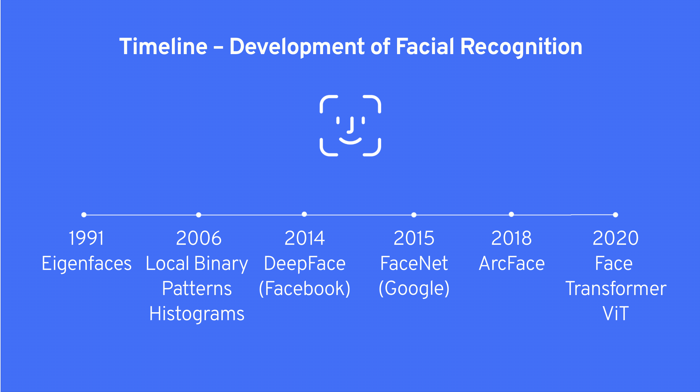
This report examines the chronological development and mechanisms behind the core evolution of deep learning architectures used for facial recognition. Here is a brief timeline of the development of facial recognition:

2. Eigenfaces

The first ever approach to facial recognition is traced back to 1991 when two researchers from MIT, Matthew Turk and Alex Pentland, introduced a Principal Component Analysis (PCA) based method to perform facial recognition without the use of any neural network. The method has been implemented in OpenCV with 97% validation accuracy on a testing set. It’s a valuable model for historical reference back when computational resources were extremely limited and deep learning was not invented yet.

There are two main biological motivations behind the invention of eigenfaces. The first one is eigenfaces’ unique feature on holistic face processing. In the human brain, the area that is used to recognise faces, the fusiform face area, recognizes faces holistically rather than by piecing together individual features like eyes, nose. Eigenfaces method does not recognize individual features but rather the face as a whole as well. The second motivation is it’s invariance to identity. Certain neurons in our brain are tuned to recognize the same face across different viewpoints, lighting conditions, and expressions while eigenfaces is also designed to execute invariance which extracts features that are characteristic of the identity of the face, regardless of various conditions. The similarity between eigenfaces features and human brain makes it the first-ever successful facial recognition model.

How it works

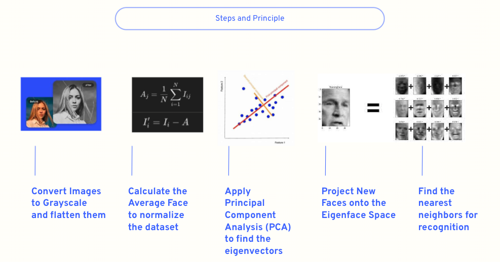
1. Convert images to Grayscale: typically, images are converted to grayscale to simplify the analysis, as color information is often unnecessary for facial recognition tasks. This step reduces the data complexity.
2. Flatten the Images: each image is then transformed into a one-dimensional vector by flattening. If an image is MxN pixels, it is reshaped into a vector of size M*N, making it easier to perform mathematical operations.
3. Calculate the Average FaceThe average face is computed by averaging each pixel across all images in the training set. This average face is subtracted from each original face image to normalize the dataset, ensuring the model focuses on the differences from the average face rather than the common features.
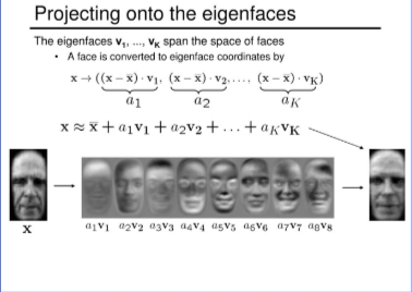
4. Apply PCA: PCA is then applied to the training images which are just subtracted by the average face which aims to reduce the dimensionality of the face image space. The idea is to find the eigenvectors (principal components) of the face dataset’s covariance matrix, which represent the directions of features wth the maximum variance in the data. These eigenvectors are the “eigenfaces.”

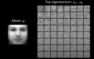
1. Project Faces onto the Eigenface Space: Each face in the training set is projected onto the eigenface space by calculating a set of weights for each face with respect to the eigenfaces. These weights form a coordinate in the reduced space, effectively capturing the essential features of the face. In other words, each face is represented by a linear combinations or a span of eigenvectors with different coefficients as shown in the photo above. The number of eigenfaces depend on the number of PCs we are choosing. All the name label is then corresponded to a coordinate in the eigenspace.

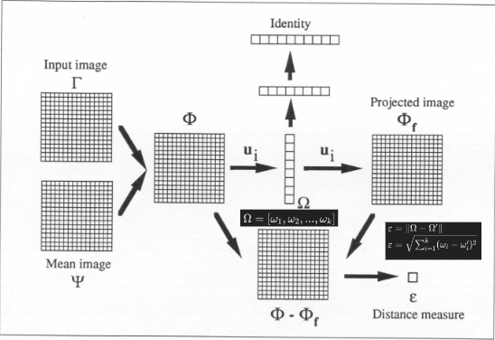
1. Recognition of new faces: For facial recognition, a new face image is processed in the same way as the training images. The identity of the new face is then determined by finding the nearest neighbors in the eigenface space based on the calculated weights.

However, comparing to the modern deep learning models, it’s accuracy fell short to those. Eigenfaces possess some obvious limitations. The most important one is it’s lack of hierarchical feature learning. PCA operates linearly and treats all variations between images equivalently without having multiple layers of abstractions to consider the hierarchical structure of facial features. The other constraints include it’s Sensitivity to non-linear Variations like certain lightning conditions and generalization of discarding some of the nuanced features that are important for distinguishing between faces that are similar.

3. FaceNet

To overcome the challenges of capturing hierarchal features which Eigenfaces faced, researchers started using deep convolutional networks for facial classification tasks.

In 2015, three Google engineers published a paper proposing a system called FaceNet, which could directly learn a mapping from an image of a face to determine facial similarity. Their method involves using a deep convolutional neural network trained directly using triplets of matching/non-matching face patches.

Model

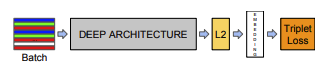
The FaceNet model structure involves a batch input layer, then a deep CNN followed by L2 normalization which gives the embedding, and then a novel loss function termed “triplet loss”.

Previous deep learning-based approaches used convolutional layers only as a bottleneck layers, which has been proven to be indirect and efficient. In contrast, FaceNet directly trains its output to be a compact 128-D embedding (essentially, the model learns an Euclidean embedding per image). The model is trained such that the squared L2 distances in the embedding directly correspond to facial similarity. With this method, verification simply becomes a task of deterimining a threshold for the distances between two facial embeddings, recognition becomes a k-NN classification problem, and clustering can be done with techniques such as k-means or agglomerative clustering.

CNN Architecture

The paper experimented with two different CNN architectures shown below. The first was one described by Zeiler & Fergus and the second was GoogLeNet.

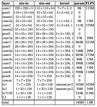
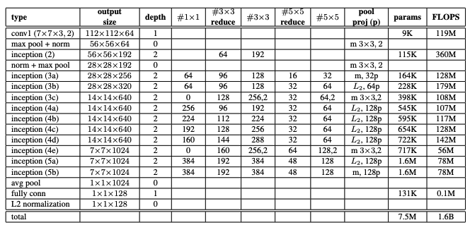
Regardless of the architecture, the CNN was was trained using SGD with standard backprop and AdaGrad. the learning rate started at 0.05 and was slowly lowered, andhe weights were initialized randomly. Both architectures showed similar results, but more commonly GoogLeNet is used.

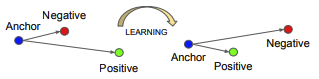
Triplet Loss

Each input is a triplet consisting of three faces: one anchor image, one positive image (matching anchor), and one negative image (not matching anchor). Triplet loss aims to minimize the distance between the anchor and positive (matching pair), and maximize the distance between the anchor and the negative (non-matching pair). The equation can be written as $ L = \Sigma^N_i[\lVert f(x_i^a) - f(x_i^p)\rVert_2^2 - \lVert f(x_i^a) - f(x_i^n)\rVert_2^2 + \alpha] $ where $x_a$ is the anchor, $x_n$ is the negative, $x_p$ is the positive, and $\alpha$ is a hyperparameter for the margin.

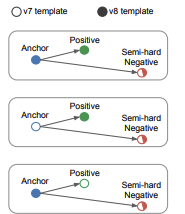
For fast convergence, we cannot use all triplets for training, so we have to only form triplets that will be effective for training. One technique is to find hard positives (postives who are far from the anchor) and hard nehatives (negatives which are close to the anchor), so the model can more efficiently learn. Another technique is to generate triplets that mix the previous iterations embeddings with the new iterations embeddings and then select the semi-hard negatives: negatives that are closer to the anchor than the positive, but still satisfy the margin, so that there is a balance between the difficulty of learning and stability in training.

A more general form of triplet loss is called tuplet loss, which can handle comparisons for more than three samples. Tuplet loss can have multiple positives and negatives in its loss calculations and attempts top optimze the emeddings amongst a wider set of comparisons.

Performance

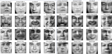
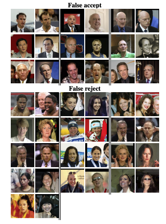
FaceNet achieved a performance of 99.63% (new record accuracy at the time) on the Labeled Faces in the Wild (LFW) dataset and 95.12% on the Youtube Faces DB. Shown below are the only errors FaceNet made on LFW.

4. ArcFace Architecture

While FaceNet introduced the triplet loss function as a way to produce embeddings, its strength tackles creating a learning model that is not subject to variation in pose, illumination, and expression. However, it hardly solves the issue with tackling the lack of discriminative power within models at the time to discriminate faces. In 2018, researcher Jiang Kang and his team at the University of Illinois published a paper titled “ArcFace: Additive Angular Margin Loss for Deep Face Recognition”, which rose to popularity through its introduction of a new loss function called Additive Angular Margin Loss (AAM) to address the limitations of traditional softmax loss as well as triplet loss.

The crux of ArcFace is to enforce discrete separations between nearest classes by modifying how feature embeddings are learned and compared. Kang referenced previous work like Sphereface as inspiration, which introduced the idea that the weights of the last fully connected layer of DCNN bear similarities to the different classes of face. Thus, ArcFace leverages a function which allows for “intra-class compactness and inter-class discrepancy”.

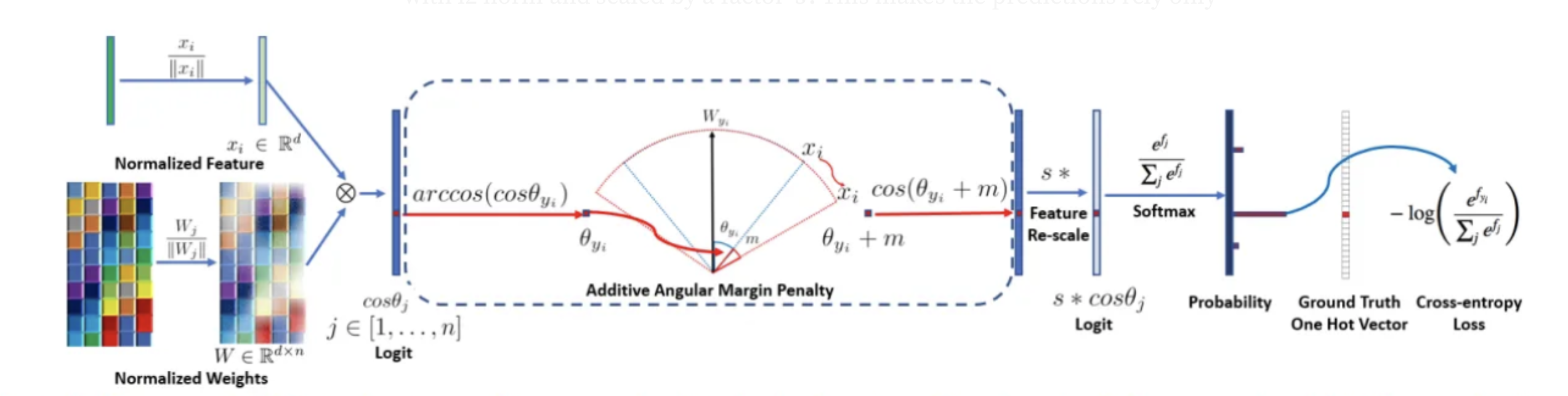
The implementation of Arcface is done by introducing an additive penalty to the dot product of the DCNN feature and the weights of the last fully connected layer. This is called the Angular Margin Loss (AML), which is calculated by taking the cosine distance between feature vectors as a metric to represent feature similarities within a geometric hyperspace. The feature vectors and the weights of the fully connected layer is then normalized to compute the cosine distance. The AML is then applied with a margin to the cosine values for the correct labels – this prevents the weights of the fully connected layer from being hyper-dependent on the input.

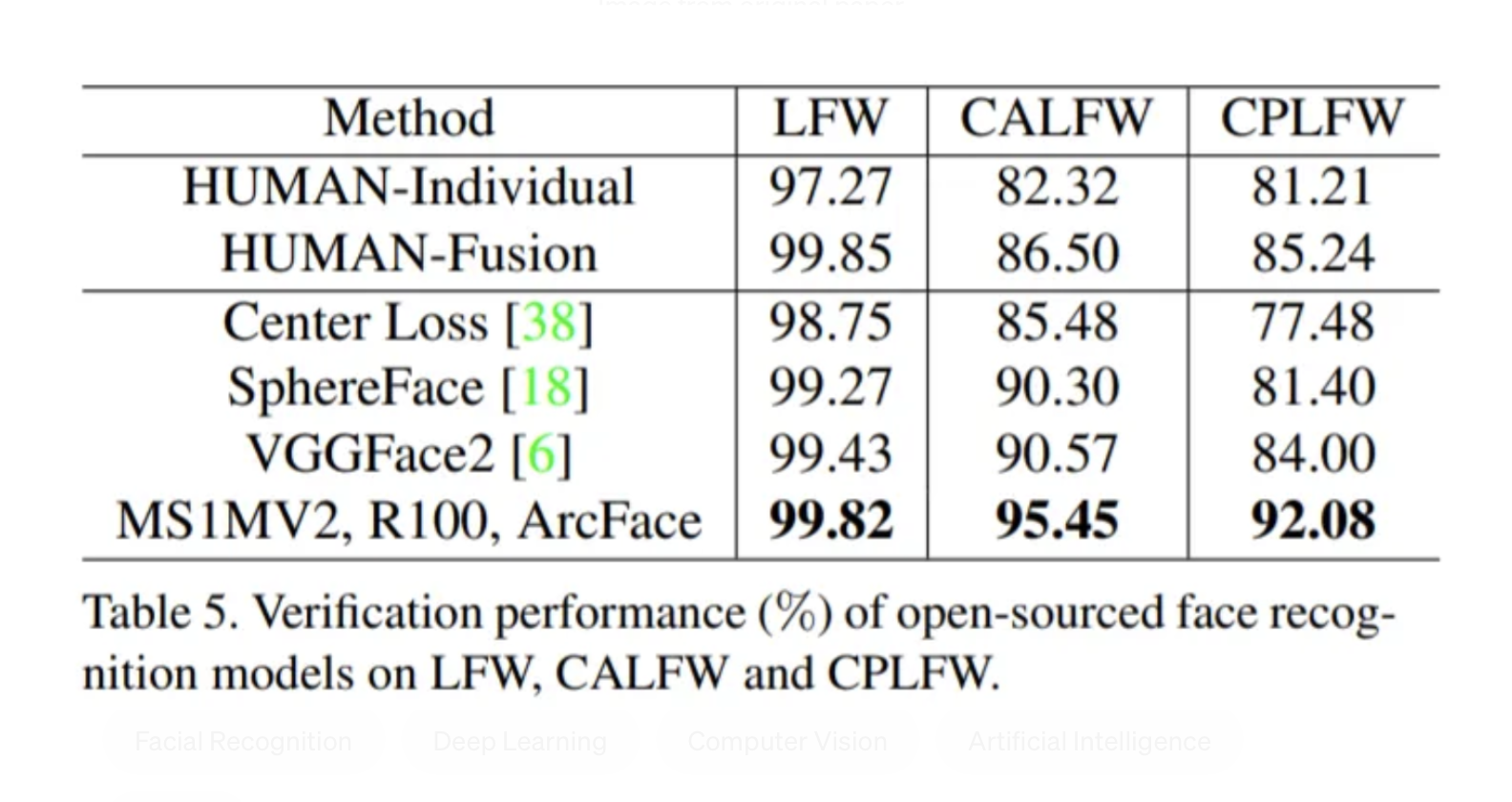
The resulting output has improved intra-class compactness and inter-class discrepancy. This is shown in Figure A, which was part of the original paper. Not only is this method more efficient than softmax loss calculations, but it also increases the reliability for facial recognition tasks greatly. When evaluating the method, the paper demonstrates that AAM performs other methodologies greatly and performs exceptionally over a variety of benchmark datasets.

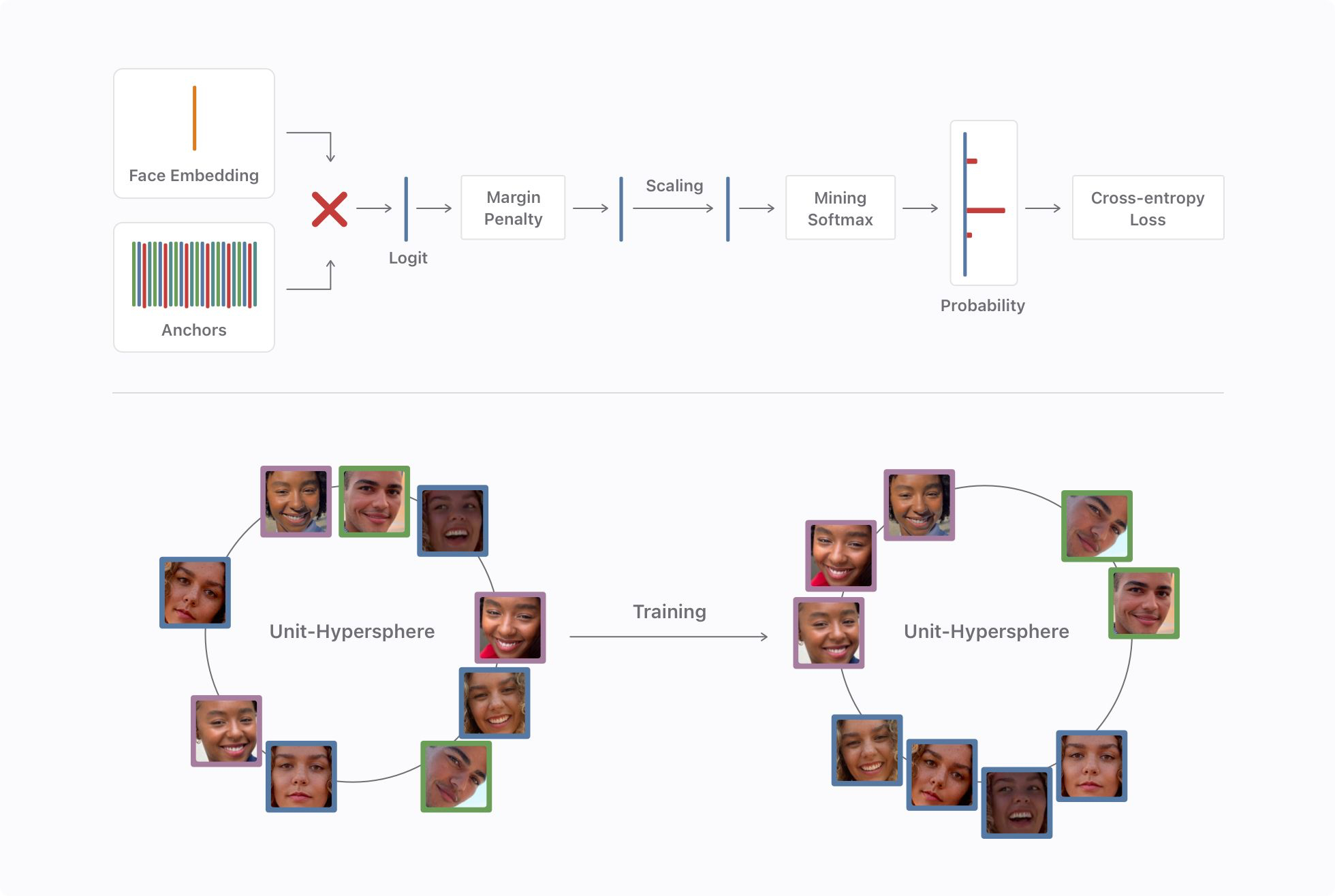
A significant moment of validation for AAM occurred when Apple’s machine learning team published an article (link) detailing their method for on-device machine learning for Facial Recognition in the Apple Photos app using a modification of AAM. During training, facial embeddings are compared and the dot-product is computed, then the additive margin penalty is added to increase the distance between different classes. The team discovered that this margin penalty technique, when coupled with their introduced “mining softmax” technique based on CurricularFace greatly improves the discriminative power of the embedding.

5. Fast Vision Transformers and Sparse ViTs

In recent years, the rise in popularity of the transformer architecture, followed by the introduction of vision transformers (ViTs) within the field of deep vision prompted an adaptation of the transformer for facial recognition tasks.

The first researchers to implement a ViT for facial classification is Zhong, Y. and Deng, W. in April 2021 (paper), where they modified the standard ViT architecture (which applies the original Transformer) and integrated the architecture within a facial recognition pipeline. The team then investigated the performance of this implementation in comparison to other pre-existing DCNN architectures that are used in real world applications. Their results showed that the ViT implementation demonstrated comparable performance with similar numbers of parameters and Multiply-Accumulate Operations in comparison to a DCNN architecture. And encouraged more research within ViT modifications to be done to enhance the accuracy of the ViT model over larger data sets.

In June 2023, research by Zhonglin Sun and Georgios Tzimiropoulos at the University of London showed the potential for part-based facial recognition to be performed by incorporating new part-based self-attention methods. Their paper, titled “Part-based Face Recognition with Vision Transformers”, introduced two new models to the field: the fViT and part fViT.

The Face ViT (fViT) is a Vision Transformer architecture that is used as a strong baseline for facial recognition using a ViT that is similar to the model proposed by Zhong and Deng in 2021, that is, using a vanilla ViT for face recognition using a vanilla loss. The increased performance is attributed to the ViT’s ability to model long-range dependencies in images, which is crucial for tasks like facial recognition where the relationship between different parts of the face can be complex and non-local.

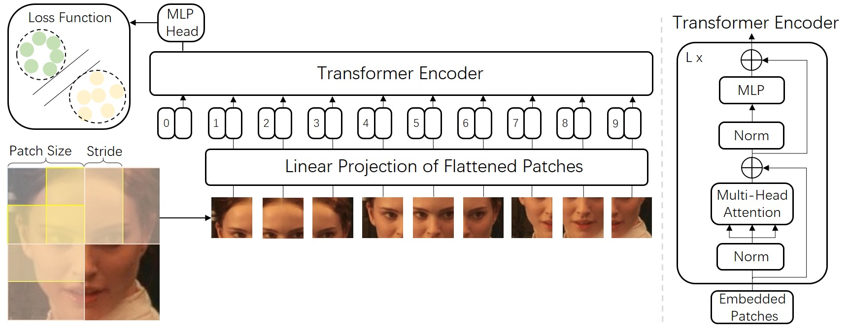
The team then capitalized on the Transformer’s inherent property to process visual tokens that are extracted from irregular grids and introduced a new pipeline for face recognition that is similar to part-based face recognition methods. The part-fViT is a lightweight network that is able to predict coordinates of facial landmarks by operating on patches that are extracted from predicted landmarks – this method of learning to extract discriminative patches, similar to the abstract model of AAM, significantly boosts the accuracy of the ViT baseline and allowed for the part-fViT to surpass many benchmarks in the field of facial recognition.

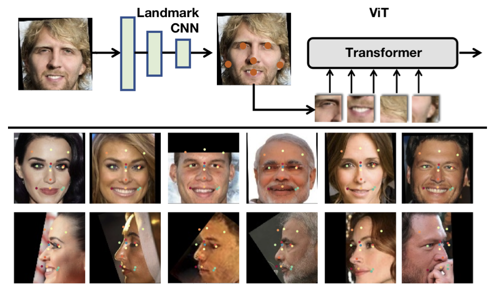
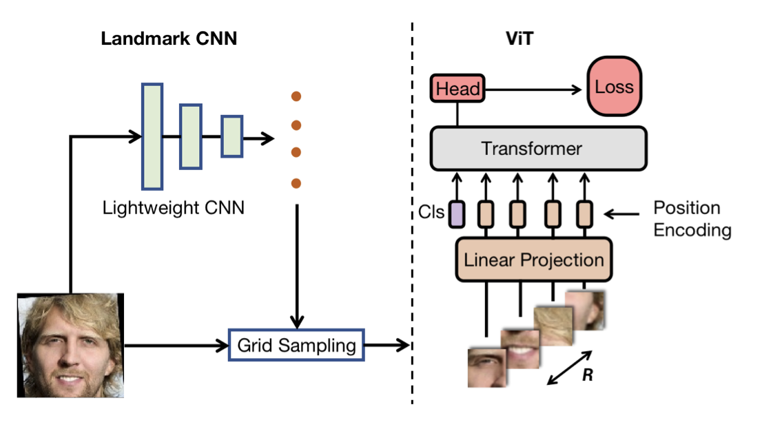
The general pipeline for the part fViT is shown in the figure above. It first uses a lightweight CNN to predict a set of facial landmarks and then a differentiable grid sampling method is introduced to extract the discriminative facial parts which are used as an input to a ViT for feature extraction and recognition.

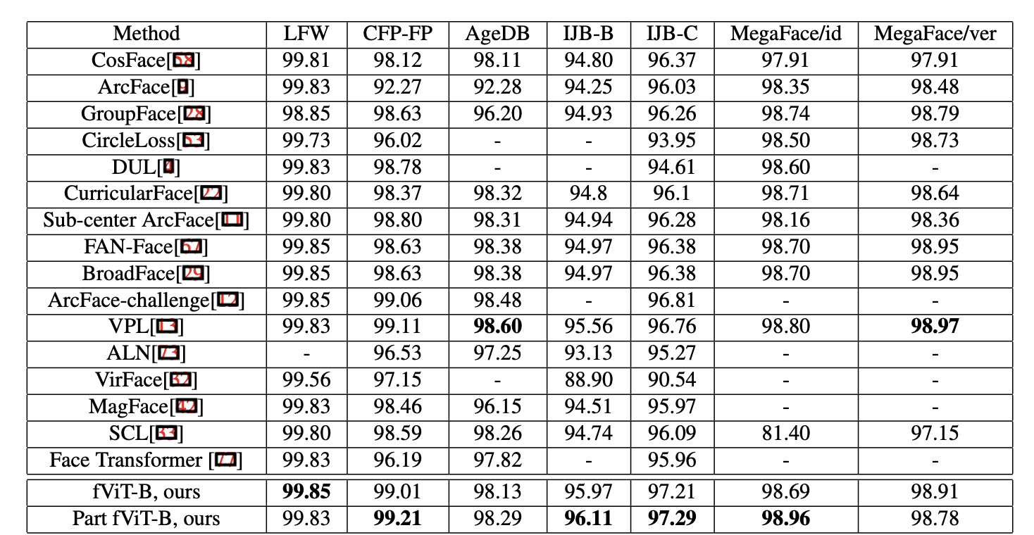
The results of the part fViT were significant – by combining the strengths of both holistic and part-based recognition methods, the part fViT surpassed most existing state-of-the-art methods.

6. Conclusion

The evolution of facial classification has significantly progressed from the inception of the eigenfaces method to the cutting-edge Vision Transformers. It all started with eigenfaces performing classification by simple PCA and without the use of any neural network, which is followed by the explosive emergence of different deep learning architectures which fully downplay the limitations from eigenfaces. Noticeably, the impressive performance of FaceNet and the innovation of ArcFace’s Angular Margin Loss signify milestones in creating more accurate and discriminative facial recognition systems. As technology marches forward, the latest adaptations in Vision Transformers indicate a promising future for the field, showcasing a robust blend of holistic and part-based methods that push the boundaries of accuracy in facial classification.

7. Our Implementation

We wanted to implement the ArcFace architecture to classify some of our own images. We found a credited GitHub repository known as InsightFace which contained implementations of the ArcFace model architecture and loss strategies.

We initially attempted to train the ArcFace model on images of our own faces. We learned how to connect a Google Cloud VM instance to our VSCode environment, so we could train the model using a GPU. However, after attempting training, we realized it would take far too long as they suggested using multiple GPUs (8) to train, otherwise it would not only take too long, but also not have great performance.

So, instead, we decided to use the insightface Python package to run gender and age detection on some of our own pictures.

import cv2
import numpy as np
import insightface
from insightface.app import FaceAnalysis
from insightface.data import get_image as ins_get_image
import onnxruntime
import os

app = FaceAnalysis(providers=['CUDAExecutionProvider', 'CPUExecutionProvider'])
app.prepare(ctx_id=0, det_size=(640, 640))

input_imgs_path = 'input_imgs'
output_imgs_path = 'output_imgs'

for file in os.listdir(input_imgs_path):
    img = cv2.imread(os.path.join(input_imgs_path, file))
    faces = app.get(img)
    rimg = app.draw_on(img, faces)
    cv2.imwrite(os.path.join(output_imgs_path, file), rimg)

Here are some of our results:

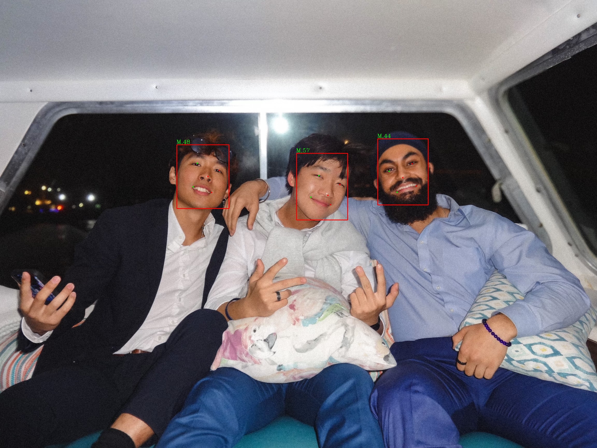
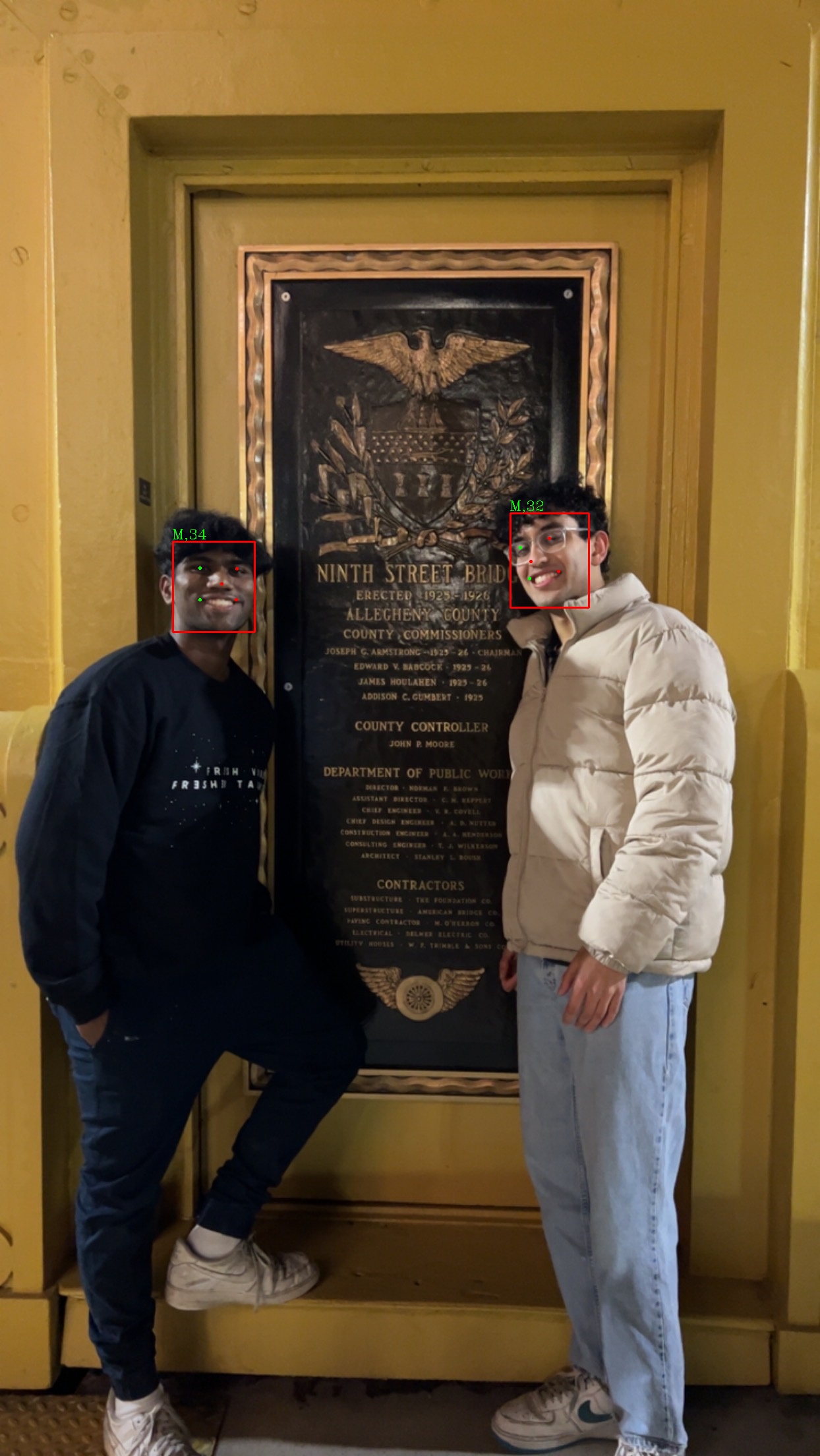
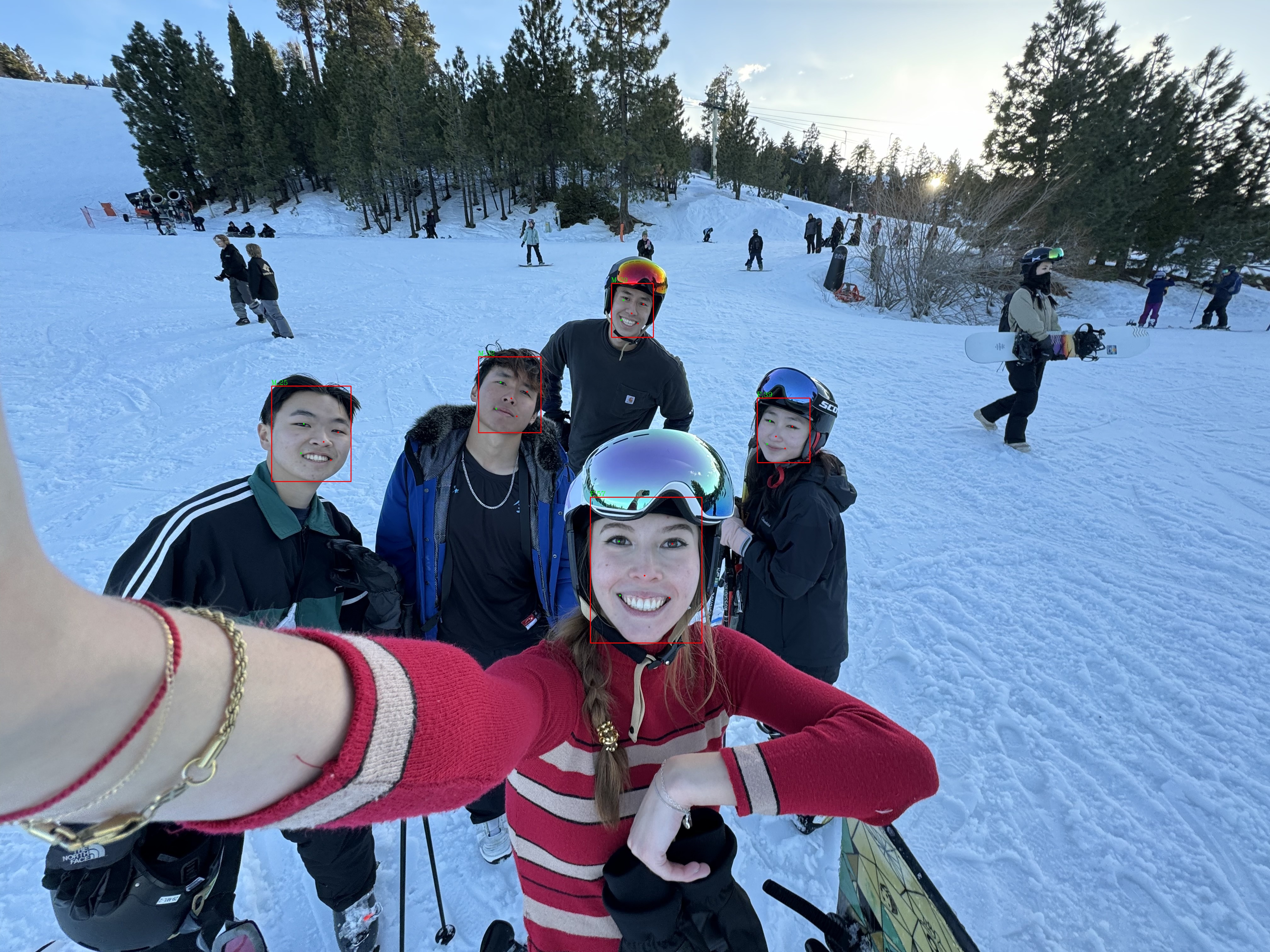
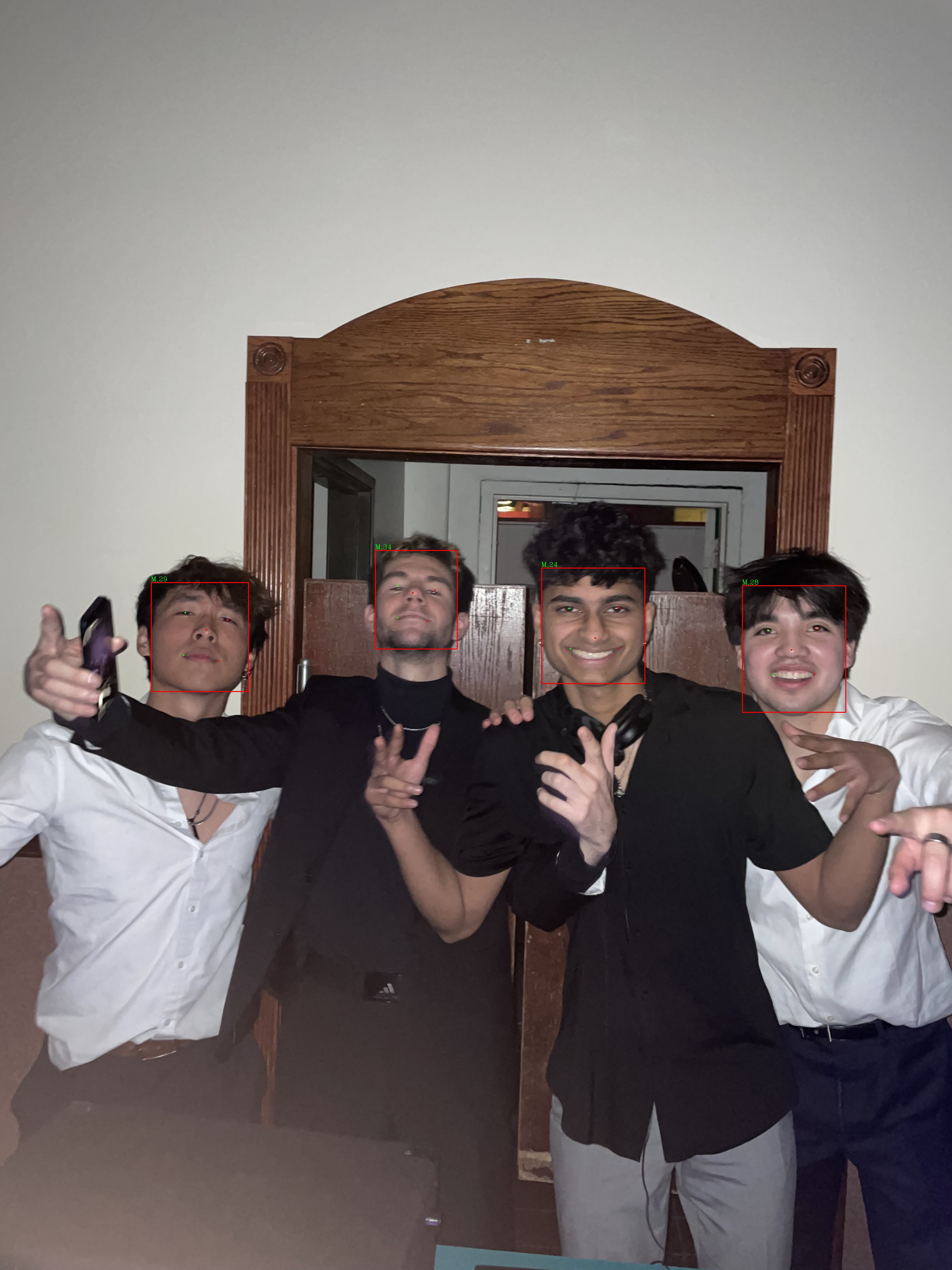
We noticed that the bounding boxes were very accurate. The age classification was not that accurate, but the gender classification had a very high accuracy. Also, the bounding box algorithm and the gender classification worked well even when people in the images were wearing helmets, covering large portions of their face and hair. ArcFace might not be able to accurately determine the age of a face because the ArcFace model is optimized for features on faces that don’t change a large amount overtime. The model is trained to maximize distinguishing features in different individual’s faces. Thus, it is not as good at determining age since age is dependent on features that can change over time. In the future, we’d like to be able to finish training their model using our images, so we can implement our own facial clustering application.

8. References

[1] Deng, J., Guo, J., Yang, J., Xue, N., Kotsia, I., & Zafeiriou, S. (2018). ArcFace: Additive Angular Margin Loss for Deep Face Recognition. ArXiv. https://doi.org/10.1109/TPAMI.2021.3087709

[2] Dupont, M. (2023, January 19). Using vision transformers for face recognition. Labelvisor. https://www.labelvisor.com/using-vision-transformers-for-face-recognition/

[3] Matthew Turk, Alex Pentland; Eigenfaces for Recognition. J Cogn Neurosci 1991; 3 (1): 71–86. doi: https://doi.org/10.1162/jocn.1991.3.1.71

[4] Schroff, F., Kalenichenko, D., & Philbin, J. (2015). FaceNet: A Unified Embedding for Face Recognition and Clustering. ArXiv. https://doi.org/10.1109/CVPR.2015.7298682

[5] Sun, Z., & Tzimiropoulos, G. (2022). Part-based Face Recognition with Vision Transformers. ArXiv. /abs/2212.00057

[6] Y. Taigman, M. Yang, M. Ranzato and L. Wolf, “DeepFace: Closing the Gap to Human-Level Performance in Face Verification,” 2014 IEEE Conference on Computer Vision and Pattern Recognition, Columbus, OH, USA, 2014, pp. 1701-1708, doi: 10.1109/CVPR.2014.220. keywords: {Face;Three-dimensional displays;Training;Face recognition;Agriculture;Solid modeling;Shape},

[7] Zhong, Y., & Deng, W. (2021). Face Transformer for Recognition. ArXiv. /abs/2103.14803

[8] Turk, M., & Pentland, A. (1991). Eigenfaces for Recognition. ArXiv. /abs/1705.02782