Computer Vision for Brain Tumor Detection

In our exploration of brain tumor classification and segmentation, we explore both 2D and 3D Convolutional Neural Networks. The brain tumor detection issue is paramount - millions of people die each year due to brain cancer, and early detection from MRI scans is integral in the prevention and aid in cancer treatment. The brain tumor classification is a machine problem, and researchers have attacked this issue in many ways, as we will elaborate on below.

• Introduction
• Classical Approach
• Modern Approaches to Classification
  • CNN-Based Brain Tumor Detection
  • Evaluation of Proposed Model
  • Grey Wolf Optimization
  • Segmentation Using 3D CNN Architecture
• Conclusions and Future Work
• Reference

Introduction

In this paper, we explore methods of detecting malignant and benign brain tumors using modern deep learning and computer vision architectures. A brain tumor occurs when abnormal cells form around the brain, and can be classified as either a malignant or benign growth. A malignant tumor - which, as it sounds, is very fatal - grows much faster than its counterpart, and may spread into a person’s nervous system. On the contrary, benign tumors grow much slower, and are very unlikely to spread to other areas. As a result, being able to classify whether a tumor is of each category is of life-or-death importance for a brain cancer patient. As machine learning architectures are evolving, there have been numerous approaches to automating this classification, to aid surgeons and doctors in cancer treatment, and to ultimately save more lives.

Classical Approach

Brain tumors are detected through imaging - through black and white MRI scans - and physical detection (the use of excisions to examine the skull and brain). MRI scans are non-invasive and critical, as they serve as the main interpreter for cancer doctors in their classification task. Today, cancer patients must wait for long periods of time to get a result back from their doctor regarding their health. These doctors also deal with another issue, other than the number of patients to look after, which is the data available regarding existing brain tumors. The combination of both these problems leads us to consider machine classification of brain tumors as our solution to patient wait times and use of historical data. However, as we are about to explore, the classification and segmentation of tumors is no easy task.

Modern Approaches to Classification

The reason for machine automation is twofold: doctors wish to first classify the tumor as malignant or benign, and segment the tumor itself given an MRI image. The first implementations of this classification faced a common issue: the lack of annotated training MRI images. In beginning approaches, researchers used single 2D black and white MRI scans, meaning image preprocessing and usage required only standardization in one channel (as opposed to RGB channels). More modern classification techniques have been trained on MRI images that emulate 3D scans - more on this later.

CNN-Based Brain Tumor Detection

The first approach we will introduce involves the use of CNNs for 2D MRI tumor detection. The researchers (Hosseini, et. al) proposed this pipeline:

1. Perform Data Augmentation to Increase Training Samples

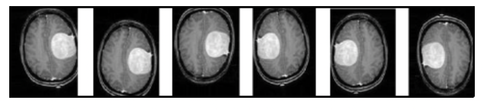
Fig 1. Augmenting existing MRI images to create extra training data [1].

The researchers mention that the original dataset used for training was only 200 images, in comparison to the thousands of images used by classic image classification architectures. To address this issue, the researchers performed rotations and changed the angle of the image, as can be seen in the figure above. The original 200 or so images became almost 1400 using this technique - for every 1 image, the researchers were able to generate 7 new images from image augmentation.

1. Preprocess Images Before Inputting into DL Model

Given that the images given to the researchers were greyscale 2D MRI scans, the preprocessing of the images before input into the CNN had three steps. First, the researchers cropped each image to get rid of unwanted black portions surround the brain. They then applied Gaussian blurring to each image to reduce the random noise, using an inbuilt function in cv2. As mentioned, they did this as the Gaussian generates a weighted average of each pixdl’s area, standardized by the standard deviation of the central pixel in the Gaussian kernel. They then performed a binary conversion to differentiate the brain (white in the scan), with the black background.

1. The CNN

The CNN architecture used by the researchers was quite elementary. They performed 2D convolution with ReLU as the activation function, then fed this output to the dense layer, which used a sigmoid function as the activation function - to perform binary classification (malignant of benign). Though the CNN was simple, the results achieved by this model were much better than its predecessors.

Evaluation of Proposed Model

For the performance evaluation of the proposed model, a BRaTS dataset consisting of class-0 and class-1 images representing non-tumor and tumor MRI images were used. Of these images, 187 were tumor (class-1) and 30 were non-tumor (class-0). These results were divided into 70-30 training splits and 80-20 training splits, and testing was performed using both of these splits.

The images underwent segmentation using image processing techniques to remove noise and standardize the images before they were passed into the classifiers for testing.

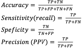
Accuracy, sensitivity (recall), specificity and precision (PPV) were used as performance metrics for evaluating the performance of the proposed model along with traditional classifiers, and were calculated using true positives (TP), true negatives (TN), false positives (FP), and false negatives (FN). These factors were calculated using the following equations:

First, traditional classifiers were evaluated using a 70:30 training-testing split and yielded the following results:

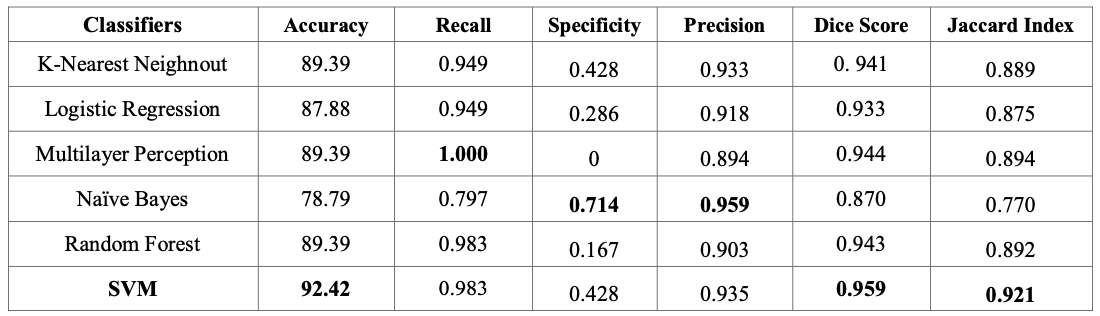
Fig 2. Performance metrics of traditional classifiers [2].

Among these traditional linear classifiers, SVM has the highest accuracy of 92.42%, but Naive Bayes provided the highest specificity value. However, this difference in precision between Naive Bayes and SVM was relatively small and written off by the authors as negligible.

The performance metrics of traditional classifiers were then compared to the performance of the proposed model. This was done in two different sets of testing, with the first set of testing utilizing the 70:30 training-testing split employed by the traditional classifiers, and a second set of testing utilizing a 80:20 training-testing split that further optimized the accuracy of the proposed model. The results of the proposed model are listed below:

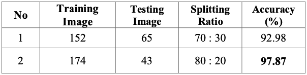
Fig 3. Performance metrics of proposed model [3].

From the results, a 92.98% accuracy aws achieved with a 70:30 training-testing split which is 0.56% higher than that of the SVM classifier used earlier. The training-testing split was further optimized into an 80:20 split and achieved an accuracy of 97.87% which is much higher than the other classifiers. During testing, experimentation was done on the number of layers in the model, but the resultant performance metrics did not show much difference given the increased complexity.

Grey Wolf Optimization

In more modern architectures, as we will see through this classification model developed by Eldin, et. al, researchers are able to leverage “3D” MRI scans to classify the existence of a brain tumor. While our last approach used a single-layer greyscale MRI image, most radiology images are given to doctors in a “3D” format - involving stacks of 2D MRI scans that resemble a higher dimensional image. This approach builds on papers like the one above in terms of increasing model accuracy during the training stage itself, which we will explore below.

The model methodology is as follows:

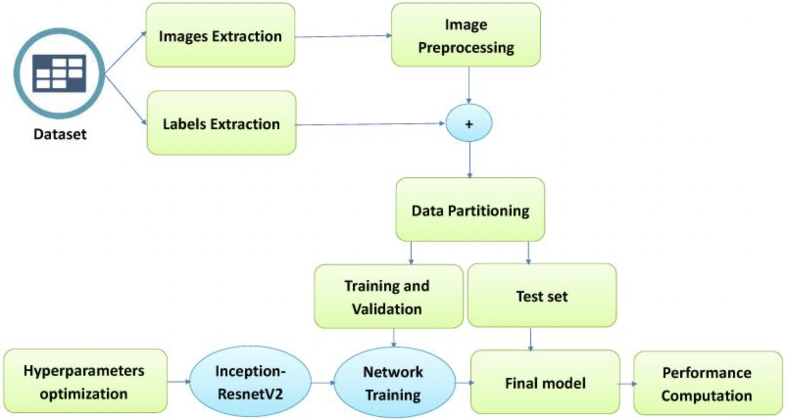
We see that the model differs from our first exploration due to its focus on hyperparameter optimization - thus lending the name “Grey Wolf.”

What is Grey Wolf Optimization?

The researchers of this approach mention that previous brain tumor classification models are able to return very high classification accuracy scores, but with a couple problems: lack of segmentation, consideration of brain position, and low accuracy. For this classification problem, a “low accuracy” is any accuracy below 99%. This is due to both the lack of training data, and the importance of classifying a malignant tumor. To address these issues, the researchers focused on hyperparameter optimization as such:

First, the hyperparemeters the researchers focused on include optimization momentum, drop rate factor, learning rate, epochs, learning rate schedule, and the L2 regularization factor - the basic hyperparameters for a CNN model.

Now for the optimization itself, the use of ADSCFGWO - or adaptive dynamic sin-cosine fitness grey wolf optimization - allows for the selection of best training hyperparameters by emulating the hierarchy of a wolf pack.

They start by initializing each “wolf” as a potential solution to the optimization problem - or a set of specific values for their hyperparameters. They then evaluate each “wolf” on the model, creating their objective or “fitness” function - the accuracy on the validation set of the data. Based on this fitness function, they take the top three wolves, and update the hyperparameter position to the direction of the “prey” - the most optimized solution. Thus, the wolves that achieve higher model accuracy “lead” the other wolves - as their hyperparameters are updated slower than the other possible hyperparameter value sets, which have to be updated more steeply to follow their “alpha wolves”. Once this grey wolf model converges, the researchers then perform their CNN-based classification - more on that below.

Segmentation of Brain Tumor Images

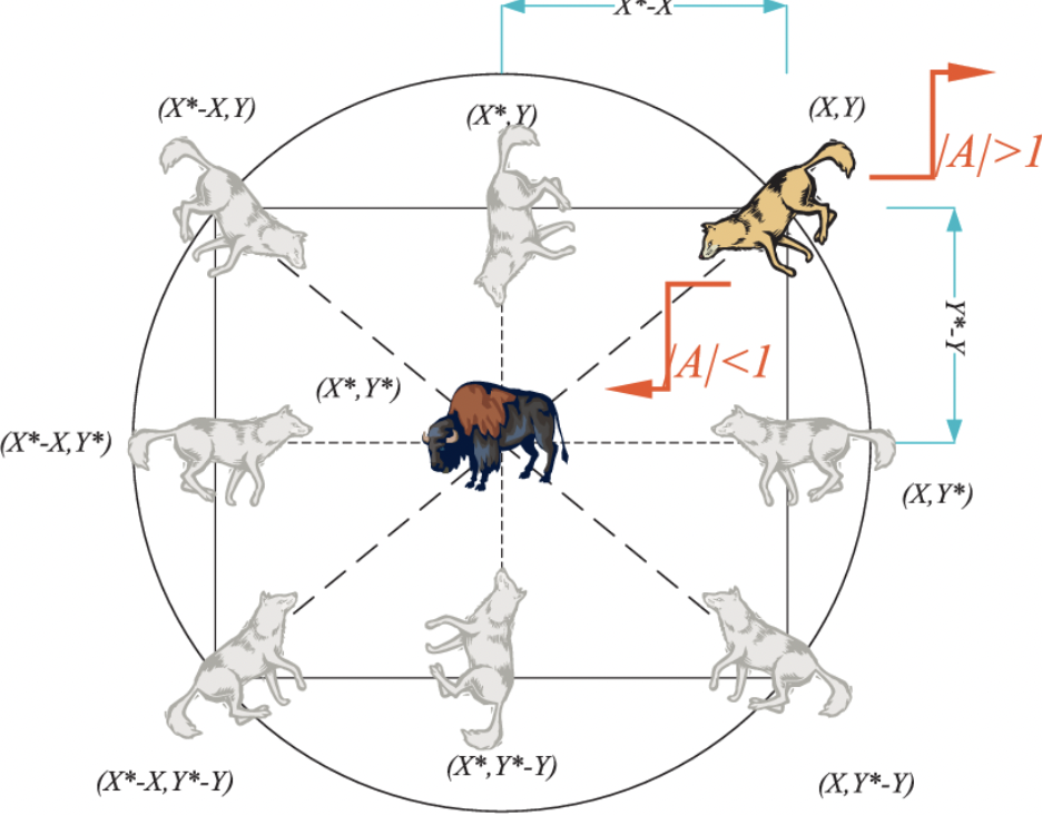
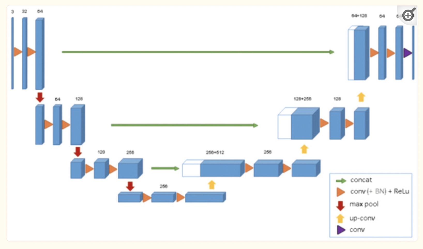Fig 4. Overview of U-Net Segmentation Architecture [4]

The researchers also tackled the lack of segmentation architecture for brain tumor imaging in their approach. By using U-Net, which is medical imaging’s most used software for imaging, to perform 3D segmentation, they were able to achieve this goal. We are able to visualize the architecture above.

Fig 5. Results of 3D U-Net Segmentation [5].

Previous 2D U-Net architectures used a similar encoder-decoder approach we learned during class. The encoder performed downsampling on the given image, using convolution layers and max pooling with stride 2, as given by the image above. The decoder or “expanding pathway” performed upsampling using transposed convolution, along with more convolutional layers and a 1x1 layer at the end to extract 64 features from the original input image for segmentation. The 3D architecture used by the researchers builds on this by using 3D convolution and max-pooling, and using batch normalization for a faster convergence and compute time.

Newer Brain Tumor Dataset

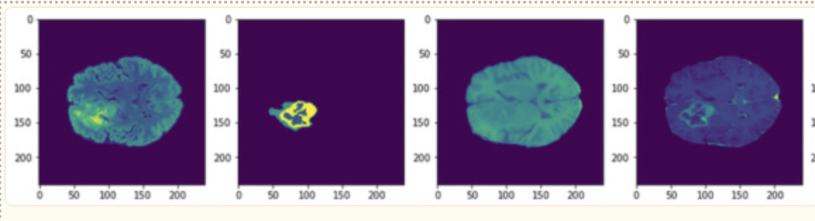Fig 6. Example of training images in the BraTS Dataset [6].

The last consideration of this paper is the availability of newer segmented imaging data. In 2021, the BraTS challenge was introduced, and a dataset of around 1200 images with annotated labels and hand-drawn segmentation data from neurologists was provided to the public. As opposed to the paper above, which started with 200 images and augmented the training dataset to include over 1200, this approach was given a much larger dataset to help prevent overfitting of data, a common issue with brain tumor detection.

Evaluation of Grey Wolf Model

The dataset used for training and testing is BRaTS 2021 Task 1 Dataset. This dataset contained clinically acquired multi-parametric MRI (mpMRI) images of gliomas, with pathologically confirmed diagnoses. To quantitatively assess the accuracy of the models, neuroradiologists created and approved ground truth annotations of tumor sub-regions for each patient in the training, validation, and testing datasets.

In the dataset, data augmentation techniques were used to artificially generate fresh training data from the aforementioned dataset. This data was augmented through image transformations including but not limited to horizontal and vertical shifts, horizontal and vertical inversions, rotations, and zooms. Image dimensions were maintained for all augmentations except inversions, which involved pivoting the pixels in the rows and the columns to produce the augmented data.

To evaluate the performance of the CNNs tested, the following metrics and calculations were used:

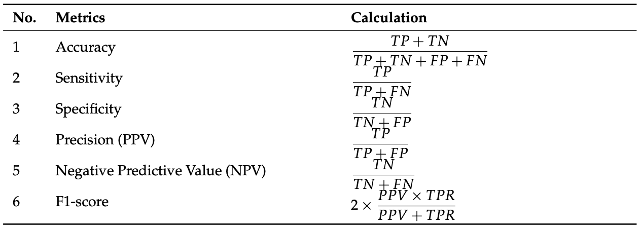Fig 7. Performance metrics used for tested CNNs [7].

Multiple CNNs were used for comparing the proposed model to current models in terms of the performance metrics above. For each of the models listed, the classifiers were run 11 times. For the proposed model (BCM-CNN), 80 iterations for 10 agents were used as hyperparameters. The results of the testing are as follows:

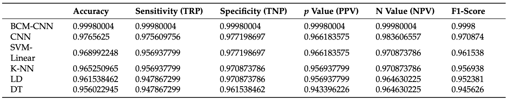Fig 8. Performance of BCM-CNN against basic classifiers [8].

Additionally, other testing was done to evaluate the stability of the algorithm involved with BCM-CNN in comparison to the other models mentioned. The researchers found that not only was the proposed model more accurate than other classifiers, but it also produced more results with accuracy in the Bin Center range than the other classifiers, indicative that multiple iterations of testing shouldn’t produce diversely different results.

Segmentation Using 3D CNN Architecture

Considerations of a 3D Network

The reseachers of our new approach, Casamitjana, et. al, propose a 3D CNN model, as opposed to the common 2D models introduced above. But in order to train a 3D model, the number of parameters and memory usage consideration is very important. The researchers focused on optimizing the depth of their network along with sampling to emulate the 2D computational performance while increasing the accuracy for 3D MRI images.

Issues with Pooling Techniques

The researchers mention that pooling techniques (such as the one used in the U-Net architecture above) do help with compute time. However, they reduce the ability of the segmentation model to capture fine-grained details. They tackle this issue by using dense inference on smaller image patches to obtain the finer features, while using convolutional layers and pooling to obtain general features for segmentation. This approach is called hybrid training.

Hybrid Training CNN (Model 1)

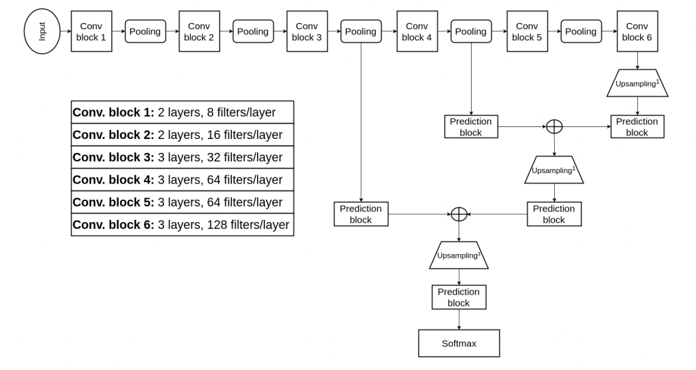Fig 9. Hybrid Training Methodology for 3D CNN [9].

As mentioned before, the researchers needed to find a way to reduce computational complexity while capturing both fine-grained and coarse features. As can be seen, there are two prediction blocks for each stage of the CNN. The prediction blocks toward the right of the model are for lower-resolution images after more pooling and convolutional layers. These blocks are used for coarse details and identifying the position of the tumor. The prediction block toward the left is used for fine-grained features, as the input image is much higher in resolution, so the CNN is able to capture texture and edges at this stage.

3D U-Net Convolution (Model 2)

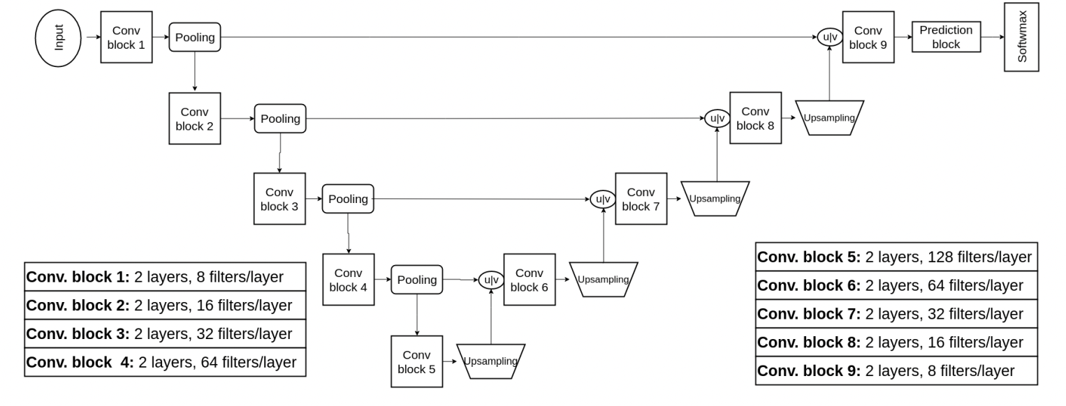Fig 10. Approach 2: 3D U-Net for Segmentation [10].

In the section on Grey Wolf optimization, we were introduced to 2D and 3D U-Net architectures for segmentation. This newer model proposed by our researchers builds on the U-Net architecture, again with the goal of capturing fine-grained and coarse features. They achieve this by concatenating the feature maps in each layer of the downsampling with their respective upsampling counterpart, as can be visualized by the “u concat v” in the diagram above. This concatenation allows the network to use contextual and local information to generate each layer output.

Evaluation of Proposed Model

The researchers in this approach used the BraTS 2016 dataset, which was much more limited than the dataset we were introduced to in the above section. This older dataset contains about 200 annotated images for each case - malignant and benign - as opposed to the 1200 images from before. As a result, the researchers did have to deal with overfitting issues, but still achieved impressive results:

Specifically, the training set consisted of 220 cases of high-grade glioma (HCG) and 54 cases of low-grade glioma (LCG) with each having ocrresponding ground truth information about the location of different tumor structures. The test set for the challenge comprised 191, with either LCG or HCG.

To evaluate the performance of segmentation methods, predicted labels were grouped in three tumor regions:

1. The whole tumor region
2. The core region
3. The enhancing core region

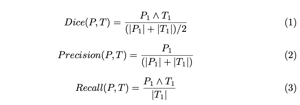
For each of these regions, Dice similarity coefficients, Precision and Recall were computed as follows:

Single- vs. multi-resolution architectures

The experiments were first carried out to compare the capability of single and multi-resolution features on the accuracy of the final tumor segmentation. Single-resolution archiectures were produced from multi-resolution architectures by taking the trained multi-resolution architectures, and cutting/skipping connections. These were compared against their base-form multi-resolution architectures leading to the following accuracy amd Dice score results:

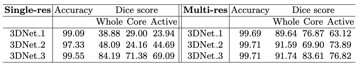
Fig 11. Results for validation set from BRaTS2016 training set [11].

Comaprison of multi-resolution architectures

The study further compares the performance of each of the three different multi-scale architectures. In general, the performance of each of the models were quite similar, with a noted trend that increasing computational costs would also marginally increase the accuracy of the model.

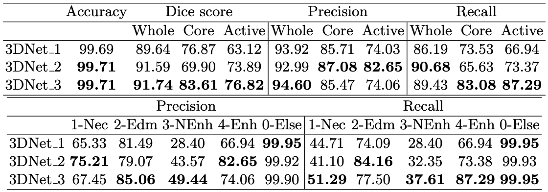
Fig 12. Results for validation set from BRaTS2016 training set [12].

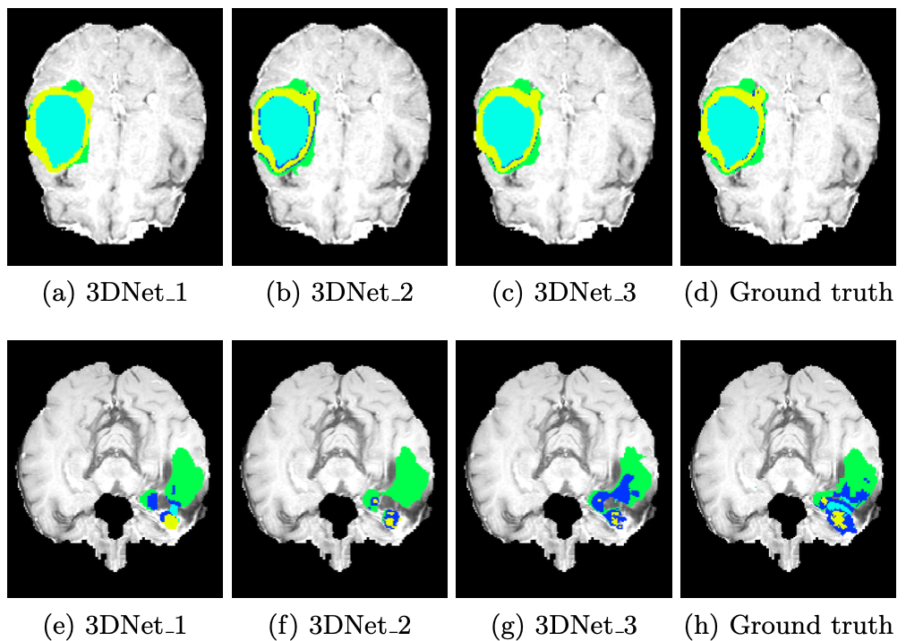
Fig 13. Qualitative comparison of results. First row has examples of large and smooth tumor regions, while bottom row samples high variability within intra-tumoral regions. [13].

However these changes were not particularly meaningful enough to fully justify that one of the models was better than the other, as the models with slightly lower computational cost and accuracy would also end up losing finer details, which might not be desirable considering the need for specificity in the field.

Conclusions and Future Work

In this article, we explore three researched deep learning methods for classifying malignant and benign tumors using MRI scans. MRI scans are crucial in medical diagnostics, offering detailed anatomical insights. The goal of implementing deep learning for this subject is to analyze these scans, aiming to distinguish between different types of brain tumors accurately.

In the first approach, a simple CNN architecture was used for brain tumor detection. Researchers used a base dataset of 200 two-dimensional MRI greyscale images. Using data augmentation techniques, this dataset was expanded to 1400 entries. In addition, preprocessing methods such as cropping, Gaussian blur, and binary conversions were used prior to training. For the architecture itself, elementary 2D convolutions and ReLU activation functions were used prior to passing the output to a dense layer and sigmoid function for binary classification. While simple and straightforward, this approach was critical to the continuing creation of machine learning based brain tumor detectors as it reached an accuracy of 97.87% with the method described.

With the proven ability of convolutional neural network architectures to accurately classify a brain tumor as malignant or benign, researchers started searching for ways to continue enhancing deep learning for increased accuracy. While a 97.87% accuracy is a notable feat, it was still deemed a “low accuracy” by many in the field because of the vast repercussions of misidentifying a brain tumor. As a result, a new goal of at least 99% accuracy was set.

In the second approach, deemed the “Grey Wolf Model”, researchers used a dataset of 1200 annotated 3D MRI Scans for brain tumor classification as opposed to the 2D scans used in Approach 1. 3D brain scans are increasingly preferred over 2D scans due to their ability to provide more comprehensive and detailed information about brain structure and abnormalities. The Grey Wolf Model focused its efforts on hyperparameter optimization for training a CNN model. In addition, the method utilized the U-Net architecture for 3D segmentation of MRI scans. Due to this focus on optimal hyperparameters prior to training, segmentation techniques, and 3D MRI scans, we saw a significant increase in accuracy compared to approach one which did not employ these techniques, as the Grey Wolf Model achieved a 99.98% accuracy. As seen, it is evident that Approach 2 considerably outperforms Approach 1. While Approach 1 helped build the foundation of using CNNs in brain tumor detection, Approach 2 focused more specifically on optimization via hyperparameters while also employing 3D training data.

In the third and final approach discussed in this article, researchers decided to also use a 3D MRI Scan dataset, although there were only about 200 annotated images. In this approach, researchers identified the problems with using pooling techniques (lack of ability to captured fine details) and proposed a new and novel architecture that included two prediction blocks for each stage of the CNN, where one is used for coarse details and identifying tumor positions, and the other is used for capturing fine-grained features. In addition, this Hybrid Training Approach builds upon the U-Net architecture by concatenating feature maps in each layer of downsampling with their respective upsampling counterparts, allowing the networks to utilize contextual and local information. The network in the Hybrid Training Approach achieved a high accuracy of 99.71%.

The Grey Wolf Model and Hybrid Training Approach differ fundamentally in the battles they are fighting. While the Grey Wolf Model is focused on hyperparameter tuning for the CNN model, the Hybrid Training Approach focuses on proposing a completely new model that combines techniques for coarse feature and fine-grained feature detection. Additionally, with the significantly smaller dataset in the Hybrid Training Approach, overfitting issues were common as opposed to the Grey Wolf Model. With the Grey Wolf Model reaching 99.98% accuracy and the Hybrid Training Approach Model reaching 99.71% accuracy, the Grey Wolf Model does appear to be the more optimal model, although the proposed ideas in both approaches have displayed significant strides in the path of using artificial intelligence for brain tumor detection.

Reference

Please make sure to cite properly in your work, for example:

[1] S. S. More, M. A. Mange, M. S. Sankhe and S. S. Sahu, “Convolutional Neural Network based Brain Tumor Detection,” 2021 5th International Conference on Intelligent Computing and Control Systems (ICICCS), Madurai, India, 2021, pp. 1532-1538, doi: 10.1109/ICICCS51141.2021.9432164. keywords: {Deep learning;Training;Speech recognition;Optical computing;Optical fiber networks;Optical imaging;Convolutional neural networks;Augmentation;Brain Tumor detection;Convolutional Neural Network (CNN);Deep Learning;Image Preprocessing;Magnetic Resonance Image},

[2], [3] T. Hossain, F. S. Shishir, M. Ashraf, M. A. Al Nasim and F. Muhammad Shah, “Brain Tumor Detection Using Convolutional Neural Network,” 2019 1st International Conference on Advances in Science, Engineering and Robotics Technology (ICASERT), Dhaka, Bangladesh, 2019, pp. 1-6, doi: 10.

[4], [5], [6], [7], [8] ZainEldin H, Gamel SA, El-Kenawy EM, et al. Brain Tumor Detection and Classification Using Deep Learning and Sine-Cosine Fitness Grey Wolf Optimization. Bioengineering (Basel). 2022;10(1):18. Published 2022 Dec 22. doi:10.3390/bioengineering10010018

[9], [10], [11], [12], [13] Casamitjana, A., Puch, S., Aduriz, A., Vilaplana, V. (2016). 3D Convolutional Neural Networks for Brain Tumor Segmentation: A Comparison of Multi-resolution Architectures. In: Crimi, A., Menze, B., Maier, O., Reyes, M., Winzeck, S., Handels, H. (eds) Brainlesion: Glioma, Multiple Sclerosis, Stroke and Traumatic Brain Injuries. BrainLes 2016. Lecture Notes in Computer Science(), vol 10154. Springer, Cham. https://doi.org/10.1007/978-3-319-55524-9_15