3D Model Generation through Machine Learning
Ever since the advent of 3D graphics, computer graphics engineers have been looking for better, more streamlined ways to create models (data representing a 3D object), a historically a tedious and long process. The goal of this post is to trace the history of 3D model generation through AI vision algorithms and suggest a potential method not just generating 3D models but pre-preparing them for use in animation and game development.
To be clear we will be discussing how AI is leveraged to generate models in a format usable by the wider 3D community. We will not be discussing algorithms that choose to represent 3D data in a form unusable by traditional animation software such as Blender, Maya or Unity (e.g. unconverted NERF data).
- Classical 3D Modelling
- Input and Output Formats
- Aside
- Learning Efficient Point Cloud Generation for Dense 3D Object Reconstruction
- Neural Radiance Fields
- Conclusion
- References
Note: This post will attempt to use the word “Algorithm” in place of “Model” to refer to Machine Learning models for clarity, due to the ambiguity of whether model refers to a 3D model or an ML model.
Classical 3D Modelling
3D graphics were a revolution when they were introduced. For the first time, computer were showing virtual world within the screen, not just flat images and text. As 3D graphics have improved, the technology has equally grown in complexity. As of the writing of this post, 3D computing has been used in simulations, movies, animation, games, and starting to grow into Virtual and Augmented reality. As a result, the need for high quality 3D computing has become a near necessity in current tech and engineering landscape.
One of the core parts of 3D graphics are models, data containing information about how to display a 3D object. The job of a 3D modeller is therefore to convert objects in the real world into 3D models such that they can be used in other applications.
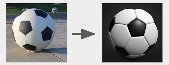
Fig 1. A real soccer ball versus it’s counterpart as a 3D model. [1] [2]
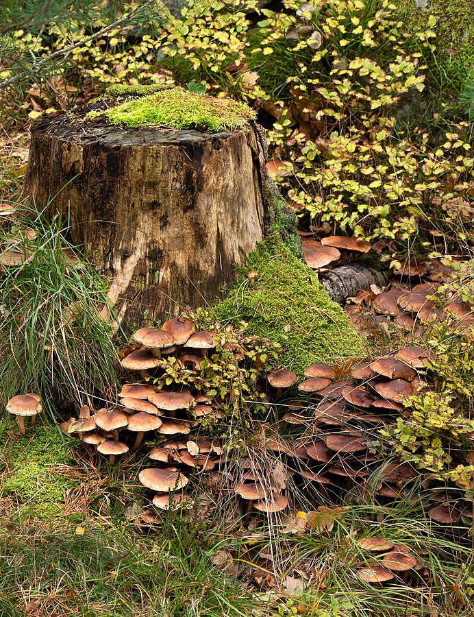
The issue with the manual creation of 3D models is time. While simple models may take a couple of hours to create, complex 3D objects with innings, concavities, minor details, etc. will take onwards of weeks to get looking right.
Fig 2. A highly detailed picture of a tree stump in an overgrown forest. [3]
Thus the question is, how can we leverage AI to speed up the process of modelling?
Input and Output Formats
Inputs
As the job of a 3D modeller is to convert real objects to 3D models, the goal of a 3D ML model is to convert an image or multiple images of an object into a 3D model. Whether we use a single image or multiple images will significantly impact how our model works and the quality of the models generated, as such it is important to consider the pros and cons of each.
Multi-Image
Multi-image models refers to the fact that the algorithm takes in multiple images of a single object from many different perspectives. The benefits of this is obvious, with more data of the object the algorithm has access to the more accurate of a 3D model it can generate. The core issue with this method is obtaining such a dataset, for large image sets of object isn’t hard to obtain, but large image sets of the exact same object are more difficult to find. To add on, multi-image data sets are also inherently less flexible for end-users, requiring them to also obtain multi-perspective images of their object while also requiring any other information the model may require of camera position data.
The most common method to generate such datasets is to take virtual snapshots of 3D models, which are significantly easier to obtain.
Fig 3. A series of images from the NeRF dataset by Ben Mildenhall, Pratul P. Srinivasan, Mathew Tancik et al. [4]
Single Image
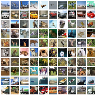
With single image algorithms, the goal is to generate a complete 3D model only using a single object in question. The immediate benefit for both the ML developer and end-user is that it is extremely simple to obtain an image of an object, as there are hundreds of millions of images on the internet. The issue for the algorithm is that it has much less data to work with, and must predict what the object’s obfuscated structure is from an understanding of spatial data and the typical structure of objects within a category.
Fig 4. A series of images from the CIFAR-10 dataset. [5]
Outputs
There are many different ways models can be stored, this post will focus on three commonly used formats by animators and game designers, point clouds, voxels, and meshes.
It should be noted that regardless of the initial format, the end-goal of all these methods is to generate a mesh. We won’t note the conversion process between these formats extensively as the conversion process is already well-defined by external, non-AI related tools, unless it is related to the algorithm being discussed.
Voxels
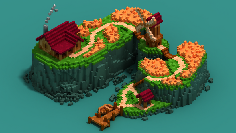
In this format, model are defined by voxels is just a collection of 3D points in XYZ space snapped to a three-dimensional grid of fixed size. These are typically the easiest to store (as they’re just lists of three numbers) and the easiest to comprehend, but doesn’t yield the best results. Due to the grid like nature of how voxels are defined, it is a trade-off between a smooth, detailed model or a space-efficient model storage-wise. However, voxel are a decent precursor to a mesh creation due to its well-defined volumes. In terms of rendering, voxels simply fill in cubes where points are defined, giving the overall model a boxy shape. While not ideal, 3D modellers are able to work with this format relatively easily by “filling in cubes”, and given certain aesthetics the “voxelated” look may even be desired.
Fig 5. Voxel art by user sebrein on DeviantArt. [6]
Point-Cloud
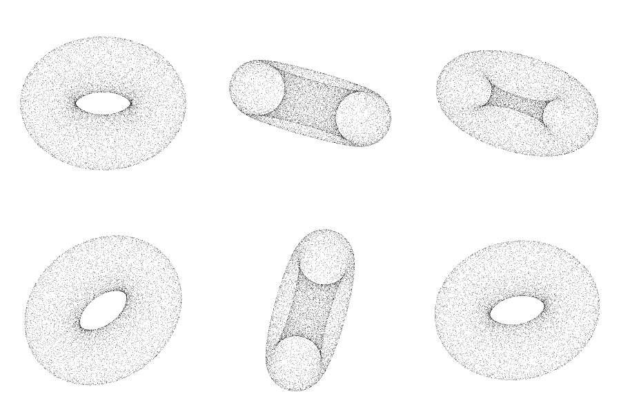
Point clouds are similar to voxels in the way that they’re also defined as a collection of points in XYZ space. However, the points in a point cloud aren’t restricted to any set grid, and therefore can exist in any place in 3D space. The trade-off for this level of detail is that point clouds don’t have a simple method to render them without some sort of conversion or lost of accuracy. For example, point clouds may be first converted to a voxel representation via rounding, then rendered that way. Another is to send a high density of ray-casts out from the rendering camera and approximating which points each ray would hit to a certain threshold. Overall though, point clouds are unideal to work with as a 3D modeller for it’s extremely hard to visualize what a point cloud would look like post-rendering, and it is highly unclear how an artist would “edit” a point cloud. The prevalence of point clouds is mainly due to the fact that it’s the best format for live capture of real-world 3D data, and as such there are many, well-developed tools that can do the conversion of point-clouds for us.
Fig 6. A point cloud representation of a torus. [7]
Mesh
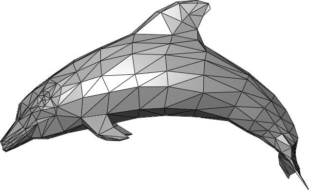
Meshes are the most common way 3D models are stored as their definition is easy to understand while giving 3D artists the greatest amount of control over the shape of a model. They are defined by three different aspects, points, edges, and faces.
Points are the simplest concept to grasp, they’re a list of discrete points that define the vertices of a 3D object. The most important data associated with points are their coordinates in XYZ space, for this data is absolutely required for the definition of a mesh’s shape. However, additional data may also be stored per point. For example, data associated with the normal of each point may be stored, which is later used to render (displaying 3D data) the object. Normals define which direction is considered “pointing” outwards at a specific point, ensuring that the model isn’t inside out and additionally can be used with interpolation to smooth the appearance of meshes without the need for more points.
Edges are edges of the 3D model, the exact same edges of a 3D shape. They’re defined as pairs of points, and typically don’t have any additional data associated with them other than the two point that define them.
Faces are the visible parts of a mesh, and the parts that are actually displayed when rendering a 3D model. They are defined by a list of points, and the normal of a face is defined as the cross product of the vectors between the points. In most meshes, faces are triangles as it significantly simplifies the calculation of face normals, defining the two required vectors for the cross product as a vector from point 1 to point 2 and a vector from point 1 to point 3. Because of this, the points that define the face must be a counterclockwise order, thus meaning that the ordering of points is extremely important.
Fig 7. A 3D mesh model of a dolphin. [7]
Aside
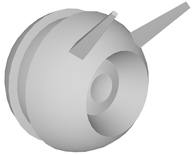
To assist with testing the different algorithms in accuracy and creativity, I introduce JC.
Fig 7. JC, our robot companion.
JC is a simple 3D model I made in blender out of a simple sphere. Their purpose is to test how accurately the following algorithms can recreate a given model, and how creative an algorithm is if they are single-image algorithms. JC will also serve as proof that these algorithms were run by me. Their obj file is linked below:
Learning Efficient Point Cloud Generation for Dense 3D Object Reconstruction
The following will be a look into a point cloud generation, single-image method developed by Chen-Hsuan Lin, Chen Kong, and Simon Lucey [9]. Their algorithm bucked the trend of 3D ConvNets that generated data in voxel grids. Instead, they sought to use point clouds, a route with the potential to run much faster and at better resolution by solely using 2D CNNs rather than expensive 3D CNNs.
Methodology
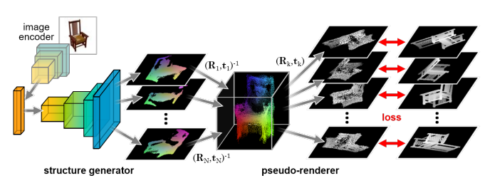
Fig 8. The network architecture of the Point Cloud Generation Network by Lin et al. [9]
There are two major portions of the network, a structure generator that generates the point cloud, and a pseudo-renderer that generates images involved in the loss-calculation of the algorithm.
Structure Generator
The structure generator follows a standard generative model architecture with opposing encoder and generator convolutional networks. The encoder first converts the input image (an RGB image) into a latent space, then attempts to generate N different depth maps from that latent space. The N different depth maps are representative what a depth map would from N different camera positions and angles. It can be visualized as a generative network that generates images of the input from a series of predefined perspectives, except that instead of each pixel having an RGB value, the pixels only have a single value called depth representing its distance from the camera, therefore representing XYZ coordinates.
These depth maps are then transformed via the known camera transformation matrices into global XYZ space, then combined into a single point cloud, the desired output of the algorithm.

Fig 9. A cropped example from the paper showing an input image and the generated point cloud by the algorithm. [9].
Pseudo-Renderer and Optimization
To evaluate the quality of the generated point cloud, the algorithm evaluates the loss between a projection of the point cloud at a fixed perspective versus a project from the same perspective of the ground truth CAD model (a specific version of a mesh 3D model). This is done as opposed to using a 3D metric (e.g. 3D distance between a 3D and a point cloud), such methods run into the issue of being too computationally expensive and therefore slow. Projections on the other hand can be compared relatively easily via traditional, 2D image loss functions. For this algorithm, the authors chose to use two loss functions, one for mask(\ref{eq:mask_loss}) (binary cross-entropy loss) and one for depth(\ref{eq:depth_loss}) (L1 loss) to optimize their algorithm.
\[\begin{align} \tag{1.1} \mathcal{L}_{\text{mask}} = \sum_{k= 1}^K -M_k \log \hat M_k - (1 - M_k) \log \left(1 - \hat M_k \right) \label{eq:mask_loss} \end{align}\] \[\begin{align} \tag{1.2} \mathcal{L}_{\text{depth}} = \sum_{k = 1}^K \left\Vert \hat Z_k - Z_k \right \Vert_1 \label{eq:depth_loss} \end{align}\] \[\begin{align} \tag{1.3} \mathcal{L} = \mathcal{L}_{\text{mask}} + \lambda \cdot \mathcal{L}_{\text{depth}} \end{align}\]To generate the projection for the point cloud, a pseudo-renderer in place of a full renderer. The point cloud is first transformed into the transform space of a selected perspective, the projected to the XY plane. The difficulty comes with conflicting points that attempt to project onto the same XY coordinates. So solve this, the rendering target space is temporarily up-sampled to a higher resolution to reduce conflicts, then a max-pooling operation on the inverse depth values (z) to down-sample the image back to the intended resolution, thereby retaining the depth values closest to the camera. Thus the algorithm can generate a projection while maintaining the ability to back propagate loss throughout the entire network (something a traditional renderer would be unable to do).

Fig 10. A visual representation of the pseudo-renderer and the effects of different up-sampling factors. [9].
Authors’ Results
This post won’t dive into every experiment ran in the paper in thorough detail. We will instead highlight the successes and potential applications of the developed algorithm.
Single Category
For single-category experiments (i.e. training on objects only of the same category, in this case chair), their algorithm was able to generate point clouds of much higher density and finer granularity than other algorithms of the time. Their takeaway from these experiments was that the explicit encoding of 3D spatial data (the pre-specified camera angles) significantly improves the efficiency and efficacy of the algorithm compared to hoping that the algorithm implicitly learned structure.
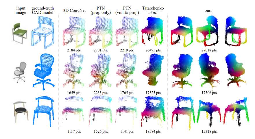
Fig 11. Single category results of Lin et al. algorithm compared to other algorithms. [9].
Visually inspecting the results of their models, it is very clear that the higher granularity significantly benefits the output of the models. Details such as the spokes of the chair are typically lost in the prior algorithms, while the author’s algorithm modelled them without any significant loss.
General Category
For general category results their algorithm similarly generated much denser results than any previous algorithm, though it is also clear the fine granularity of the algorithm was lost. For thin structures, the model had a difficult time filling the areas in with a high enough density and finer details seemed to be lost entirely. However, overall it does preform better at these tests than competing algorithms at the time.
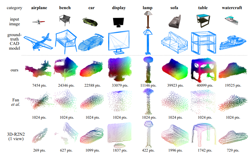
Fig 12. General category results of Lin et al. algorithm compared to other algorithms..
Out Attempted Experiments and Issues
The intention of this section was to recreate the results from the algorithm and test it with novel data. However, it seems that the repository holding the author’s original code has fallen into disrepair. Attempts were made to port it to newer versions of TensorFlow and have it run on newer hardware, but unfortunately all attempts led to corrupted data. Below is proof that an attempt was made.
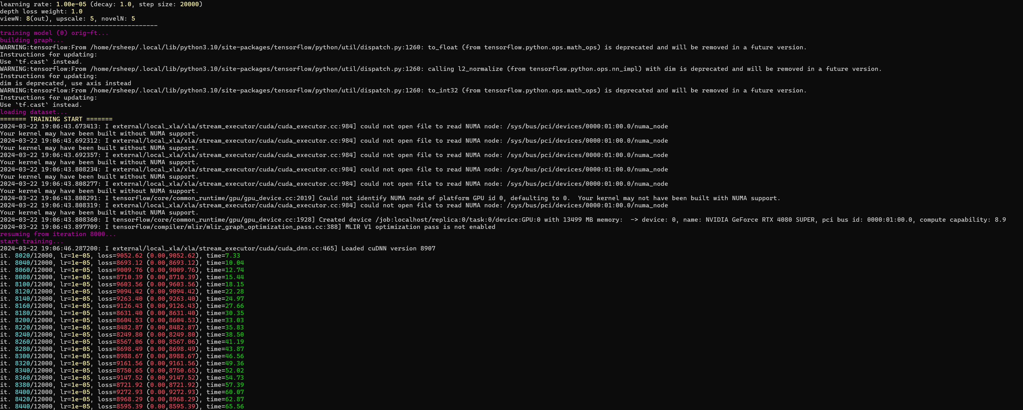
A converted version of the algorithm that was auto converted somewhat by the TensorFlow v1 to v2 algorithm running on Windows WSL, CUDA version 11.8, cuDNN version 8. [9].
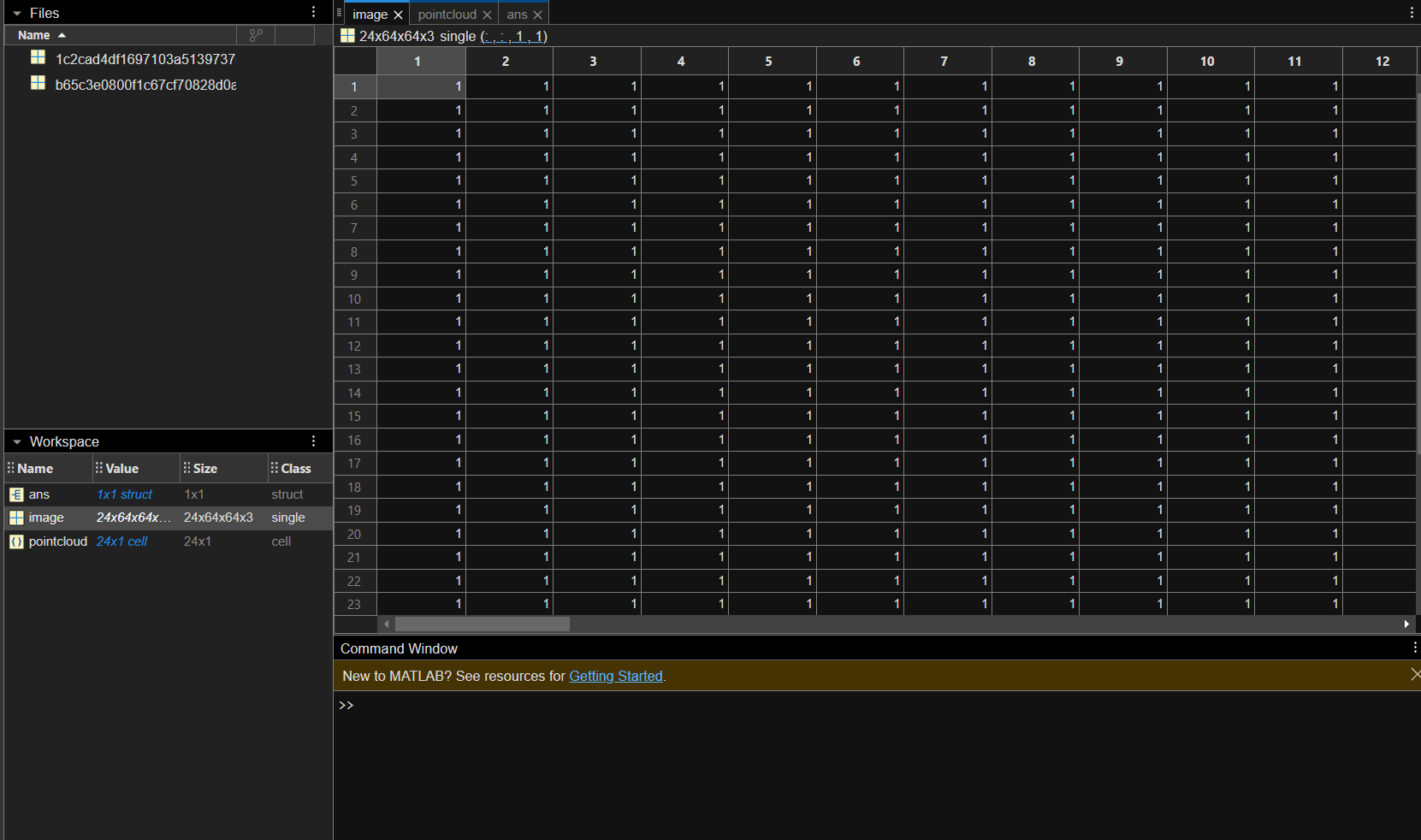
One of the resulting data files outputted by the model, which were all in the form of MatLAB. Due to typing errors information was indecipherable.
Given enough time an effort, it would be possible to either upgrade the author’s code to Tensorflow V2 or recreate the proposed algorithm from scratch, though with the advent of much better algorithms as the one we will discuss next, it may be best to keep this as a historical landmark in the progress toward better 3D model generation.
Neural Radiance Fields
The next portion will look into a more recent algorithm developed by Ben Mildenhall, Pratul P. Srinivasan, Mathew Tancik et al. that utilizes neural radiance fields to render scenes from new perspectives. The algorithm is a multi-image, requiring multiple images from various perspectives to generate its output, a neural radiance field capable of being converted to a mesh via a marching cubes algorithm. The main benefit of this method is the consideration of full volumetric data rather than solely surface data, allowing for novel views that consider occlusion, transparencies, and reflections.
Methodology
The central idea of NeRFS is remarkably simple. Given a set of 5D points that define XYZ position in space along with two angular coordinates $\theta$ and $\phi$ representing the viewing angle. These points are randomly sampled along rays that extend outwards from the camera/perspective position, one ray per pixel of each image. These points are then fed into a MLP network that outputs a color and density of each point.

Fig 13. A representation of each step of the NeRF algorithm. [10].
Once trained, \(F_\Theta\) is essentially a function that returns the color and density at any given point in 3D space given a certain orientation. Thus when rendering a new perspective, the idea is that (similar to when learning) a grid of rays is emitted from the camera position we wish to render the radiance field from. Each ray then takes a series of sample points along it, which returns an RGB and density value per sample point. The values returned are then accumulated to return the final RGB value of that pixel (\ref{eq:accum}), thus resulting in a rendered image from a novel view that not only considers what the perspective is looking at, but how orientation effects aspects such as specularity, transparency, and occlusion of the object.
\[\begin{equation} \tag{2.1} \hat C(r) = \sum_{i=1}^N T_i (1 - \exp(-\sigma_i \delta_i)) c_i, \:\: \text{where } T_i = \exp\left(-\sum_{j=1}^{i-1} \sigma_j \delta_j \right) \label{eq:accum} \end{equation}\]Loss and Optimization
Two notable optimizations were also implemented to improve the speed and quality of the resulting outputs.
The first of which is positional encoding. It was discovered in a different paper by Rahaman et al. [11] that mapping inputs to higher dimensional space improves the performance of algorithms that have high-frequency variation (significant output differences from minor changes in input). Thus, they leveraged positional encoding to scale up the dimensionality of their input data, a mapping typically used in Transformer architecture to provide positions of tokens used in the input. In this case however, it is solely used to increase dimensionality.
\[\begin{equation} \tag{2.2} \gamma(p) = (\sin(2^0 \pi p), \cos(2^0 \pi p), \cdots, \sin(2^{L-1} \pi p), \cos(2^{L-1}\pi p)) \label{eq:pos_enc} \end{equation}\]The other optimization is hierarchical volume sampling. The key issue with doing a single sample along the ray is that many of the samples will be relatively useless for the overall calculation of the radiance field as the sample may land on a point where there is either empty space or a position that is occluded. Thus, rather than raising the sampling rate to try to capture more information, two sampling passes are used. A first coarse sampling is used to get a general sense of which densities are relevant along a ray. After that, a second sampling is taken that adjusts the sampling density to focus on points of higher density in the coarse pass, thus giving higher granularity to the most relevant parts of the ray.
\[\begin{equation} \tag{2.3} \hat C_c (r) = \sum_{i=1}^{N_c} w_i c_i, \:\: w_i = T_i(1- \exp(-\sigma_i\delta_i)) \end{equation}\]The above equation would be the first, coarse pass, as where the prior equation, \(\hat C (r)\) would be the fine pass.
Finally, the loss function is relatively simple, where the coarse and fine passes are both compared to the ground truth image, both using L2 loss functions.
\[\begin{equation} \tag{2.4} \mathcal{L} = \sum_{r \in \mathcal{R}} \left[\left\Vert \hat C_c (r) - C(r) \right\Vert_2^2 + \left\Vert \hat C_f (r) - C(r) \right\Vert_2^2 \right] \end{equation}\]Author’s Results
It is unnecessary to say that the results of NeRF are visually amazing. A video demonstrating their results is shown below.
Overall the resolution and accuracy of these interpolated views is stunning to say the least. The algorithm generates views that are near flawless even studied up close.
The greatest issue for the purposes of this post however is the quality of their meshes.
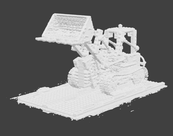
Fig 13. A mesh generated from NeRF data. [10].
Here they used a typical marching cubes algorithm to generate the model, which to give them credit is leagues above what we’ve seen so far. The issue is noise, as finer details get lost in the noise of the NeRF data. Normally for image generation, these aspects are smoothed out by the fact that it’s an image, but when converted to modelling, it is far from perfect.
Our Results (CS188 Assignment 4)
The following is a summary of Assignment 4 of CS188, which included PyTorch implementation of the NeRF algorithm. An attempt was made to run the code directly from the paper’s authors, however there were issues with getting TensorFlow working. The only change was increasing the resolution of the training images.
Credit goes to the original authors of the homework assignment, assumed to be Zhizheng Liu and Tian Yu Liu. If there was an author of which the assignment was adapted from, credit would then go to them, though after research and issues with the number of variations of the exact same project, it was indeterminate who created the first Jupyter Notebook implementation of NeRF.
Ray Generation and Sampling
As in the original algorithm, a grid of rays is generated for each given perspective of the training set, which will be later used to generate color and field density.
def get_rays(H, W, focal, c2w):
    i, j = np.meshgrid(np.arange(W), np.arange(H), indexing='xy')

    # transform the image coordinates to world coordinate system
    dirs = np.stack([(i-W*.5)/focal, -(j-H*.5)/focal, -np.ones_like(i)], -1)
    rays_d = np.sum(dirs[..., np.newaxis, :] * c2w[:3,:3], -1)
    rays_o = np.broadcast_to(c2w[:3,-1], rays_d.shape)
    return np.stack([rays_o, rays_d], 0)
The following PyTorch module defines the MLP that the NeRF algorithm uses to transform spatial coordinates and angle to RGB values and density. The only difference between this implementation of MLP versus a typical implementation is the lack of a final activation, for we want the unaltered output values to represent some sort of function f(x,y,z,\(\theta\),\(\phi\)) = (R, G, B, D).
import torch.nn as nn
import torch
from torch import optim
class SimpleNeRFMLP(nn.Module):
    def __init__(self, in_dim, net_dim, num_layers):
        super(SimpleNeRFMLP, self).__init__()
        # create a list to store the layers of the MLP
        ############# Your Implementation here #############
        # Your tasks:
        #    1. Create a fc layer with in_dim as input and net_dim as output.
        #    2. Create (num_layers - 2) fc layers, all with `net_dim` in and `net_dim` out,
        #          and ReLU activation function.
        #    3. Create a final fc layer with `net_dim` number of input features
        #         and 4 output features (1 density channel + 3 RGB channels).
        #         ###Don't use any activation here####
        # Hint: You can use torch.nn.Sequential to link your layers together

        self.fcFirst = nn.Linear(in_dim, net_dim)

        self.fcs = nn.ModuleList()
        for i in range(num_layers - 2):
            self.fcs.append(nn.Sequential(
                nn.Linear(net_dim, net_dim),
                nn.ReLU()
            ))

        self.fcLast = nn.Linear(net_dim, 4)

        ############# End of Your Implementation #############


    def forward(self, x):
        out = None
        ############# Your Implementation here #############
        # Implement the forward pass, taking in a coordinate 'x'
        # as input, and returning the density and RGB value for that coordinate
        # in variable 'out'

        out = self.fcFirst(x)
        for f in self.fcs:
            out = f(out)
        out = self.fcLast(out)

        ############# End of Your Implementation #############
        return out
Lastly is the code block which replicates the coarse and fine sampling that the author’s used in their original algorithm.
def render_rays(
    model, num_freq_bands, rays, near, far, N_samples, rand=False):
    # super long comments...
    """
    Renders an image from 3D rays by first uniformly sampling points along each
    ray, encoding these points using positional encoding, and then computing the
    predicted color and opacity at each point using the given MLP model.

    Args:
    model (nn.Module): MLP model that takes encoded 3D points as input and
            returns the predicted color and opacity.
    num_freq_bands (int): Number of frequency bands used for positional encoding.
    rays (Tuple[torch.Tensor, torch.Tensor]): Tuple containing origin and
        direction of the rays. Both tensors are of shape (num_rays, 3).
    near (float): Near clipping plane distance.
    far (float): Far clipping plane distance.
    N_samples (int): Number of samples along each ray.
    rand (bool): Boolean indicating whether to add random noise to jitter training points.

    Returns:
    Tuple[torch.Tensor, torch.Tensor, torch.Tensor]: A tuple containing:
    - rgb_map (torch.Tensor): Tensor of shape (num_rays, 3)
          containing the predicted RGB color for each pixel in the image.
    - depth_map (torch.Tensor): Tensor of shape (num_rays, )
          containing the predicted depth for each pixel in the image.
    - acc_map (torch.Tensor): Tensor of shape (num_rays,)
          containing the accumulated alpha (transmittance) for each pixel in the image.
    """
    rays_o, rays_d = rays
    # uniformly sample points in the space from near to far.
    interpolations = torch.linspace(
        near, far, N_samples, device=rays_o.device).repeat(rays_o.shape[0], 1)
    if rand:
        # add random noise to jitter training points
        interpolations += (torch.rand(
            list(rays_o.shape[:-1]) + [N_samples], device=rays_o.device)
                  * (far-near)/N_samples) # we need to scale the noise accordingly

    # sampled pts in 3D space
    pts = rays_o[...,None,:] + rays_d[...,None,:] * interpolations[...,:,None]
    pts_flat = torch.reshape(pts, [-1,3])

    # Apply positional encoding to pts_flat
    pts_flat_freq_encoded = pos_enc(pts_flat, num_freq_bands).float()
    raw = model(pts_flat_freq_encoded)
    raw = torch.reshape(raw, list(pts.shape[:-1]) + [4])

    # Compute opacities/occupancy and colors
    rgb, sigma_a = raw[...,:3], raw[...,3]
    sigma_a = torch.nn.functional.relu(sigma_a)
    rgb = torch.sigmoid(rgb)

    # Do volume rendering
    # delta
    dists = torch.cat([interpolations[..., 1:] - interpolations[..., :-1],
                       torch.full_like(interpolations[...,:1], 1e10, device=rays_o.device)], -1)
    # alpha
    alpha = 1.-torch.exp(-sigma_a * dists)
    # transmittance
    trans = torch.where(1 - alpha > 1., 1., 1.-alpha + 1e-10)
    trans = torch.cat([torch.ones_like(trans[...,:1]), trans[...,:-1]], -1)
    # weights
    weights = alpha * torch.cumprod(trans, -1)

    rgb_map = torch.sum(weights[...,None] * rgb, -2)
    acc_map = torch.sum(weights, -1)
    depth_map = torch.sum(weights * interpolations, -1)
    return rgb_map, depth_map, acc_map
The dataset we used was the tiny NeRF dataset originally included in the repository of the author’s code, but now can be found hosted at this link http://cseweb.ucsd.edu/~viscomp/projects/LF/papers/ECCV20/nerf/tiny_nerf_data.npz.
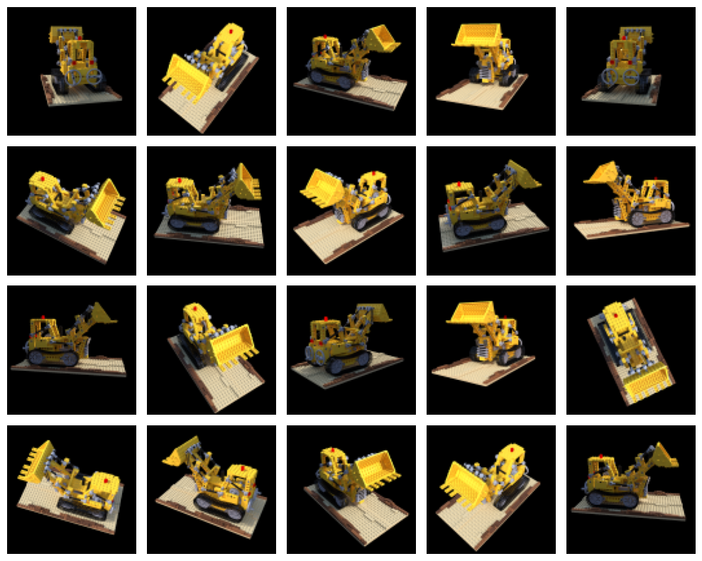
Fig 14. Randomly sampled images from the yellow tractor dataset. [10].
Fig 15. Result of NeRF model, sampling perspectives of a full 360 degrees around the truck.
Conclusion
Overall, the clear trend of 2D image to 3D model generation seems to be heading in the direction pioneered by NeRF. However, within the intuition of how NeRF works we can see the same techniques utilized by older, point cloud methods. For example, the use of varying perspectives to train off projections of the model and camera raycasting are carried over from point cloud methods to NeRF algorithms.
Further algorithms have already built off of the work the author’s of NeRF made, for example a newer 2023 paper by Yicong Hong et al. [11] has already created an LRM algorithm that generates full, high quality models from a single image, combining image encoding, NeRF, and image to tri-plane algorithms to achieve their results. Commercial implementations of these algorithms already exist, though I will not be linking them here. Overall the field of image to model generative algorithms seems extremely promising from a technical stance.
A short aside from an artist’s perspective
This short blurb comes from me personally, and is a short opinion piece rather than a technical breakdown. As exciting as this technology is as a tech enthusiast, the creative in me worries about the worrying implications these algorithms have. Specifically when it comes to misuse, as I wish to make it clear that I firmly believe that these algorithms, as mentioned in the introduction should be used to improve the work of 3D artists, and not replace them. These algorithms should be treated as a quick way to generate templates, a starting point to work off of rather than using their outputs as is. The prior algorithms in this list (to my knowledge) seem to acquire their datasets ethically, which I cannot say the same for commercialization of LRM algorithms. This blurb is a cautionary piece to note that as exciting as ML is, it is important to remember they rely on the work of real people who take the time to learn and perfect their craft. Without them, there would be no data to train out algorithms off of, and if we eliminate them, there will be no more data to further train our algorithms with. As AI enters the creative space, all I ask of future ML engineers reading this post is to treat others with respect, especially the artists, photographers, writers and more that have taken the time to create the data you use.
References
[1] “Soccer Ball” by tinmanjuggernaut is licensed under CC BY 4.0
[2] “Giant Soccer Ball” by A. Scott Fulkerson / Circle Jerk Productions (TM) is licensed under CC BY-SA 4.0
[3] “Mushrooms by a tree stump 5” by W.carter is in the Public Domain, CC0
[4] B. Mildenhall, P. P. Srinivasan, M. Tancik, J. T. Barron, R. Ramamoorthi, and R. Ng, “NeRF: Representing Scenes as Neural Radiance Fields for View Synthesis.” arXiv, 2020. doi: 10.48550/ARXIV.2003.08934.
[5] Krizhevsky, A., Nair, V. and Hinton, G, “The CIFAR-10 Dataset” University of Toronto, 2014. https://www.cs.toronto.edu/~kriz/cifar.html
[6] “Farming island isometric voxel art” by sebrein is licensed under CC BY-ND 3.0
[7] “Point cloud torus” by Lucas Vieira is in the Public Domain, CC0
[8] “Dolphin triangle mesh” by Chrschn is in the Public Domain, CC0
[9] C.-H. Lin, C. Kong, and S. Lucey, “Learning Efficient Point Cloud Generation for Dense 3D Object Reconstruction.” arXiv, 2017. doi: 10.48550/ARXIV.1706.07036
[10] B. Mildenhall, P. P. Srinivasan, M. Tancik, J. T. Barron, R. Ramamoorthi, and R. Ng, “NeRF: Representing Scenes as Neural Radiance Fields for View Synthesis.” arXiv, 2020. doi: 10.48550/ARXIV.2003.08934.
[11] Y. Hong et al., “LRM: Large Reconstruction Model for Single Image to 3D.” arXiv, 2023. doi: 10.48550/ARXIV.2311.04400.
