Novel View Synthesis
In this article, we take a deep dive into the problem of novel view synthesis and discuss three different representative methods. First, we examine the classical method of light fields rendering, which involves learning a 4D representation of a scene and applying multiple compression techniques. We then jump into Neural Radiance Fields (NeRFs), a modern deep learning approach that has achieved much better visual clarity and memory usage by implicitly modeling scene representations with a neural network. Our discussion of NeRFs’ drawbacks will lead us to the emergence of 3D Gaussian Splatting (3D-GS), an effective rasterization technique that explicitly encodes a scene with thousands of anisotropic gaussians.
- Introduction
- A Classical Approach: Light Fields
- Neural Radiance Fields (NeRFs)
- 3D Gaussian Splatting (3D-GS)
- Experiments
- Conclusion
- Reference
Introduction
The task of novel view synthesis involves generating new scene views given a limited set of known scene perspectives. Solving this problem can open the doors to recinematography, refined virtual reality, quality scene representations, and more. Successes in this area have primarily sprouted from recent machine learning approaches, namely neural radiance fields (NeRFs) and 3D gaussian splatting (3D-GS).
In this article, we give an overview of both a classical and deep learning approach and discuss their pitfalls in order to motivate 3D gaussian splatting, an approach we will investigate in detail.
A Classical Approach: Light Fields
One of the most prevalent classical methods for novel view synthesis is by representing a scene with light fields. These light fields are 4D representations of a scene’s radiance as a function of the light ray’s position and direction.
Light Slabs are defined by the function: \(L(u, v, s, t)\), where \(u, v, s, t\) are values that describe two coordinate systems. The idea is that given two 2D planes in space, a ray in the scene will intersect each plane at exactly one point. By defining the first plane with coordinates \((u, v)\) and the second plane with \((s, t)\), we can uniquely describe a ray with these four coordinates [1].
To learn all the function \(L(u, v, s,t)\), we make use of the many different angles captured of a scene. Each view will then contain many rays described by the \(u, v\) and \(s, t\) coordinates, and the corresponding radiance will be mapped. Then, to synthesize a new view, a novel 2D slice can be taken. By placing a new camera in the scene, rays can be projected from the scene onto to this camera coordinate system, which is denoted as a set of rays \({R_1, R_2, ..., R_N}\). Each ray \(R_i\) is defined by the coordinates \((u_i, v_i, s_i, t_i)\) and the radiance is mapped to the pixel.
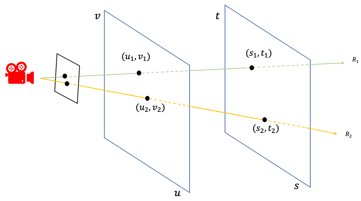
Fig 1. Light field visualized. [1]
Pros and Cons
The main benefit of using this traditional method for novel view synthesis is that it doesn’t reqiure lots of memory and can be easily implemented on workstations and personal computers. Although storing the actual light fields themselves would require gigabytes of data, a comprehensive compression pipeline helps solve this issue. In particular, they first use vector quantization to store a limited number of reproduction vectors. Through vector quantization, the compression rate is around \((kl)/(log N)\), where k is the number of elements per vector, l is the number of bits per element (typically 8), and N is the number of reproduction vectors [1]. The second stage of the compression pipeline is an entropy coder, with the goal of reducing the cost of representing high cost indices. Many scenes involve a similar or constant colored background, and so by applying an entropy coder algorithm like gzip or Huffman coding, the representation can further be reduced by a factor of 5. Due to this compression pipeline, the light field method for novel view synthesis has lower memory requirements than the deep learning techniques described later in this article.
There are three main downsides to this approach. First, to create an accurate representation of the field, we need many unique views of a scene. If there a lack of viewing angles, the learned function \(L(u, v, s, t)\) may be inaccurate, and result in poor syntheses. Second, the light fields method struggles with scenes that involve occlusion. This type of scene tends to be challenging, and recent research have explored methods to improve performance of Light Field based view synthesis involving deep learning methods. Lastly, for light fields reconstruction to work, there needs to be a fixed source of illumination. As the 4D light field representation is learned with a particular illumination equation, we can have multiple light fields each with their own illumination equation and stitch the outputs of each field respectively. However, this method would require more memory usage as well artifacts from inaccurate stitching, which can be better solved with other methods. In general, the light fields classical method results in low resolution reconstructions as shown below, and recent works have applied deep learning methods to achieve better performances.
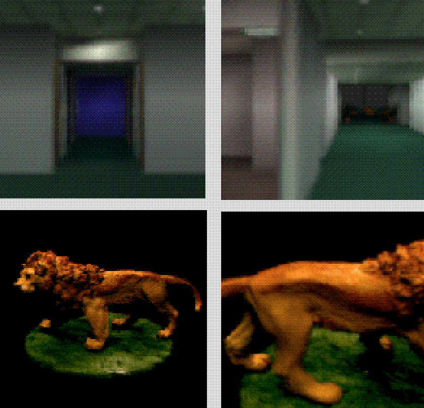
Fig 2. Novel View Synthesis using Light fields visualized. [1]
Neural Radiance Fields (NeRFs)
On a high level, NeRFs aim to optimize a continuous volumetric scene function \(F_\theta\) that essentially implicitly encodes a scene representation. More formally, the input of \(F_\theta\) is a spatial location \((x, y, z)\) and viewing direction \((\theta, \phi)\) and the output is the predicted volume density \(\sigma\) and view-dependent emitted radiance [2].

Fig 5. Neural Radiance Field diagram. [2].
NeRF Algorithm Overview
- Generate rays from known camera poses and collect query points.
- Train 3D scene representation with MLP.
- Input location and viewing direction of query points.
- Predict color and volume density.
- Render based on each ray’s volume density profile.
- Compute loss between rendered image and ground truth image.
Generating Rays and Query Points
Given a collection of camera poses, we want to first generate a set of rays originating from the camera center and intersecting each pixel of the image plane.
We can denote each camera pose as \(v_o = (x_c, y_c, z_c)\), where \(x_c, y_c, z_c\) encapsulates the camera center in world coordinates. We can also represent each ray as a normalized vector \(v_d\). Now, we can construct a parametric equation \(P = v_0 + t \cdot v_d\), which defines points along our ray from a certain camera view.
The next step is to determine the set of query points for training. There exists many approaches for this subtask with the simplest being uniform sampling, in which we simply take \(n\) equally-spaced points along the ray. Immediately, one may realize the complexities involved in constructing such a ray sampler. We want to be able to not only sample across the relevant object space within a scene but also sample more frequently in areas of higher volume density. In light of these considerations, the original authors introduce hierarchical volume sampling, which allows for adaptive sampling based on high-density areas.
Network Architecture
At this point, we have obtained a set of query points (locations + viewing directions), which we can input into a multi-layer perceptron (i.e. fully connected network) and predict the color and volume density. The architecture used in the original paper is depicted below:
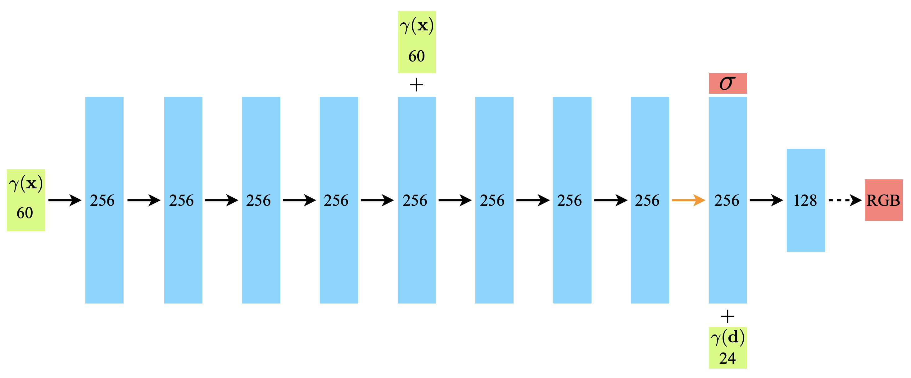
Fig 3. NeRF MLP architecture. [2].
The main thing to note is that at first only the positional information (along with their fourier features) is inputted into the network. The viewing angle information is only injected after view-independent volume densities are predicted. With this added context, the network can then finally output a view-dependent RGB color.
Positional Encoding
It turns out that training with the raw positions and view directions is not sufficient for the network to encode a high-quality scene representation. The original authors explained this issue as the result of the internal bias within neural networks to learn low frequency functions.
This motivates us to transform the raw input into a higher-frequency space. This is done by concatenating Fourier features to the input to obtain the following input feature vector:
\[\gamma(p)=\left(p, \sin\left(2^0 \cdot p\right), \cos\left(2^0 \cdot p\right), ...,\sin\left(2^{L-1} \cdot p\right), \cos\left(2^{L-1} \cdot p\right) \right)\]Hierarchical Volume Sampling
As mentioned before, we’d like to make our sampling process efficient by adaptively sampling more points in high-density areas. To accomplish this, two models are constructed: one coarse and one fine. The coarse model uniformly samples along each ray and its output is used to determine areas of high-density. The fine model then adaptively samples based on the coarse model’s results. The outputs of the fine model are used for the final rendering.
Image Formation Model
To obtain the image formed at some viewing direction, NeRF uses an approximation to the traditional volume rendering method, which can be written as:
\[\hat{C}(\textbf{r}) = \sum_{i = 1}^N c_i \alpha_i \prod_{j = 1}^{i - 1} (1 - \alpha_j)\]where \(\alpha_i = 1 - \exp(-\sigma_i \delta_i)\).
This equation essentially describes a weighted mean of all the colors along the ray of interest. These colors are weighted by the volume density at that point and transmittance, which represents how much light has been transmitted in the ray already. The transmittance weighting is \(T = \prod_{j = 1}^{i - 1} (1 - \alpha_j)\).
Loss Function
With both coarse and fine models, the basic loss function for NeRFs is defined as:
\[\mathcal{L} = \sum_{\textbf{r} \in \mathbb{R}}(\lVert \hat{C_c}(\textbf{r}) - C(\textbf{r}) \rVert _2^2 + \lVert \hat{C_f}(\textbf{r}) - C(\textbf{r}) \rVert _2^2)\]where \(\hat{C_c}(\textbf{r})\) are the predictions from the coarse model and \(\hat{C_f}(\textbf{r})\) are the predictions from the fine model [3].
Pros and Cons
The NeRF model marked a huge breakthrough in novel view synthesis and was a cornerstone algorithm. Compared to previous SOTA methods at that time, it thoroughly outperformed those methods in terms of image quality and memory usage. In the original NeRF paper, they tested benchmarks against other single network methods such as SRN, NV, and LLFF (Local Light Field Fusion). While SRN and NV both train a separate neural network for each scene, LLFF uses a pretrained 3D convolutional network to predict discretized frustum-sampled RGB\(\alpha\) grids.
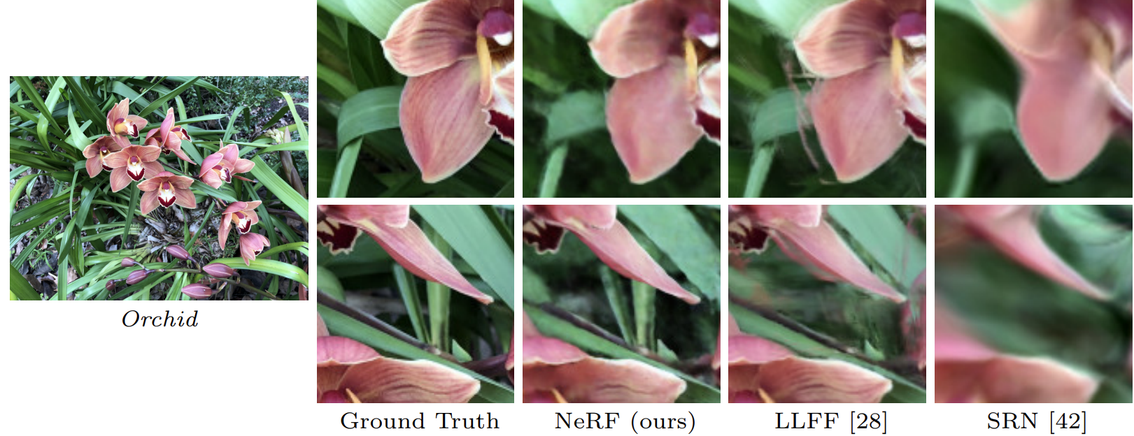
Fig 4. NeRF reconstruction vs LLFF and SRN. [].
As shown in the example above, NeRF tends to render more detailed reconstructions when compared to previous baselines (fern leaves are less blurry and orchid patterns better match the ground truth). Additionally, NeRFs are able to much more accurates capture occluded parts of the scene, such as in the yellow shelves in the fern crops, especially when compared to LLFF methods and SRN. Aside from enhanced visual reconstruction, NeRFs also require much less memory than LLFF, which produces a large 3D voxel grid for each image. On the other hand, NeRFs only need to store the weights for the neural network. For reference, the memory requirement for one “Realistic Synthesis” scene is 15GB when using LLFF and only 5 MB for NeRF.
The main downside of NeRF compared to previous methods such as LLFF is the training time required. Neural network methods such as SVM and NV take at least 12 hours to train for a single scene, while LLFF reduces this time to only 10 minutes. If applications where fast or real time synthesis is required, methods such as light fields or Gaussian Splatting (to be explained later) may be preferred to NeRFs.
3D Gaussian Splatting (3D-GS)
Before diving into the details of this approach, we first need to discuss core computer graphics concepts that are essential to this technique.
Rasterization
Rasterization is the process of drawing graphical data onto a rasterized (pixelized) screen. In computer graphics, objects are commonly represented by simple polygonal faces like triangles. Each of these polygons are decomposed into pixels and rasterized into a raster image.
Gaussian splatting is essentially a rasterization technique. Instead of rasterizing simple polygons, we rasterize 3D gaussian distributions. Each of these gaussians can be described by its position (mean, \(\mu\)), splat size (covariance matrix, \(\Sigma\)), color (spherical harmonics), and opacity (\(\alpha\)). Mathematically, it can be expressed as follows:
\[G(x) = \frac{1}{2 \pi \lvert \Sigma \rvert^{\frac{1}{2}}} e^{-\frac{1}{2} (x - \mu)^T \Sigma^{-1} (x - \mu)}\]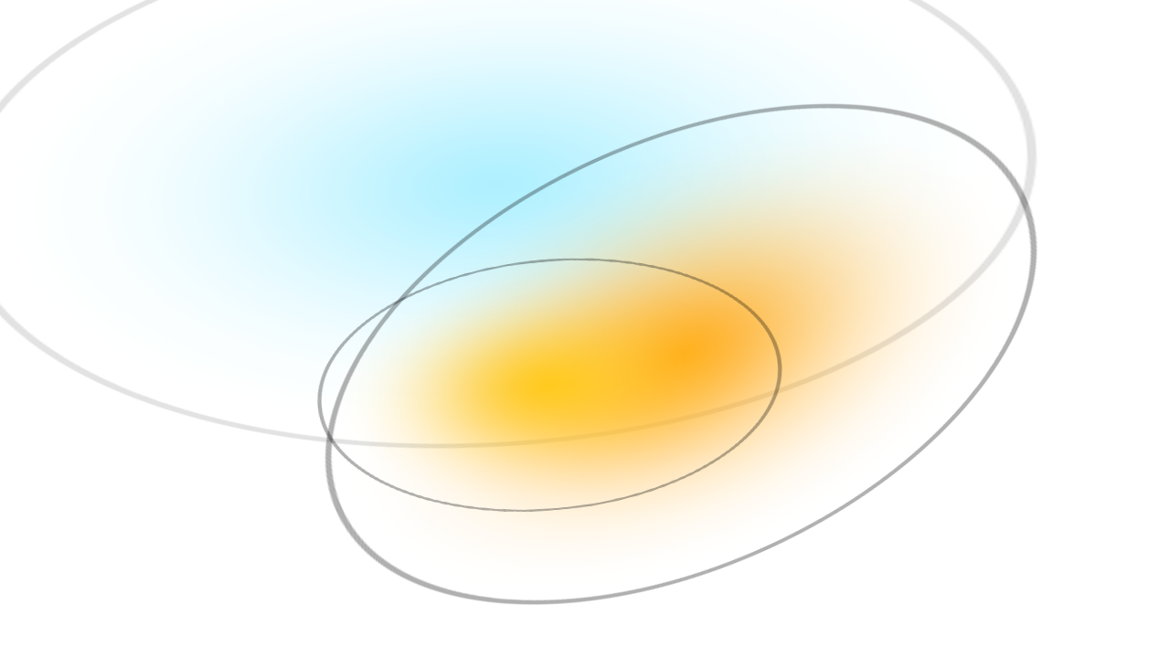
Fig 5. Gaussian splat visualized. [6].
So, in other words, we can learn an efficient representation of a 3D scene as a composition of thousands of 3D gaussian distributions. How does this process work? Let’s take a look!
3D-GS Algorithm Overview
- Given a set of images, estimate a pointcloud with Structure from Motion (SfM).
- Initialize isotropic gaussians at each point.
- Train 3D scene representation.
- Rasterize gaussians with a differentiable rasterizer.
- Compute loss between raster image and ground truth image.
- Adjust gaussian parameters with SGD.
- Densify or prune Gaussians.

Fig 6. 3D Gaussian Splatting pipeline. [4].
Pointcloud Estimation
Our first objective is to determine a rough scene structure. This is accomplished by using Structure from Motion, a method based on stereoscopic photogrammetry, to construct a pointcloud.
The algorithm at its core works by detecting and tracking keypoints across a sequence of scene view images using various feature detection and extraction techniques, such as SIFT and SURF. Then, camera poses are estimated and 3D positions of keypoints are triangulated.
Initialization of Gaussians
After pointcloud generation, we initialize an isotropic gaussian at every point. Isotropic means that these gaussians have diagonal covariance matrices. The mean of the gaussians are also set to the average of the distances to the 3-nearest neighbors. This initialization approach is both intuitive and performs well empirically.
Differentiable Rasterizer
The training process begins with processing the gaussians into a differentiable rasterizer.
- Project each Gaussian into 2D camera perspective.
- Sort Gaussians by order of depth.
- Perform front-to-back blending of Gaussians at each pixel.
Projection
In any rasterization procedure, we must take our objects that lie within the 3D world space and project them into the 2D image space. For the differentiable rasterizer, we would like to compute the mean \(\mu\) and covariance \(\Sigma\) of every 3D gaussian projected into 2D.
Before we derive these computations, we first define the instrinsic camera matrix \(K\) and the extrinsic camera matrix \(W\) as follows:
\[K = \begin{bmatrix} f_x & 0 & c_x \\ 0 & f_y & c_y \\ 0 & 0 & 1 \end{bmatrix}\] \[W = \begin{bmatrix} r_{11} & r_{12} & r_{13} & t_x \\ r_{21} & r_{22} & r_{23} & t_y \\ r_{31} & r_{32} & r_{33} & t_z \end{bmatrix}\]where \(f_x, f_y\) are the focal lengths and \(c_x, c_y\) describe the camera center.
We can then compute the 2D projection of our homogeneous gaussian mean \(\vec{\mu}\).
\[\begin{bmatrix} u \\ v \\ z \end{bmatrix} = K W \vec{\mu}\] \[\begin{bmatrix} u \\ v \\ z \end{bmatrix} = \begin{bmatrix} f_x & 0 & c_x \\ 0 & f_y & c_y \\ 0 & 0 & 1 \end{bmatrix} \begin{bmatrix} r_{11} & r_{12} & r_{13} & t_x \\ r_{21} & r_{22} & r_{23} & t_y \\ r_{31} & r_{32} & r_{33} & t_z \end{bmatrix} \begin{bmatrix} \mu_x \\ \mu_y \\ \mu_z \\ 1 \end{bmatrix}\]To get the projected mean \(\vec{\mu}^{2D}\), we need to perspective divide to obtain the 2D coordinates.
\[\vec{\mu}^{2D} = \begin{bmatrix} u / z \\ v / z \end{bmatrix}\]Now, we want to compute the 2D projection of our covariance matrix \(\Sigma\). It was straight-forward to compute the projected gaussian mean. Covariance, on the other hand, will require some further intuition.
The perspective projection is a non-linear transformation, which when means that the 3D gaussians are no longer true gaussians in the 2D projection. So, we would like to approximate the projection by linearization such that we obtain true gaussians in the projection space.
This linear approximation can be done using the Jacobian of the projection matrix, denoted as \(J\). It follows that the covariances in camera coordinates are \(\Sigma^{2D} = J W \Sigma W^T J^T\), where \(W\) encapsulates the world to camera transformation.
Rendering
Once projection is complete, we now have a set of 2D gaussians (represented by the projected means and covariances). So, it remains to compose the final rendered image using an image formation model, which turns out to be quite similar to the one used in NeRFs.
Recall that in a NeRF, the image formation model can be formulated as:
\[C(p) = \sum_{i = 1}^N c_i \alpha_i \prod_{j = 1}^{i - 1} (1 - \alpha_j)\]For gaussian splatting, we have:
\[C(p) = \sum_{i = 1}^N c_i f_i^{2D}(p) \prod_{j = 1}^{i - 1} (1 - f_j^{2D}(p))\]Despite the resemblance of their equations, the difference in computing \(\alpha_i\) and \(f_i^{2D}(p)\) are actually at the core of gaussian splatting’s stronger performance. In NeRFs, we have to query a MLP at every point to determine the volume density and emitted radiance, which will essentially give us \(\alpha_i\). On the other hand, in guassian splatting, we’re able to precompute all projected gaussians and directly use them at every pixel (i.e. we avoid unnecessary reprojection of gaussians).
Rasterizer Optimizations
An important advantage of gaussian splatting is its fast rendering time when compared to alternative deep learning methods such as NeRF. One of the largest reasons for this is the fast differentiable rasterizer. The main goals with this rasterizer is to have fast overall rendering and sorting to allow for approximate alpha-blending and avoid hard limits on the number of splats that can be learned [4]. The key steps of the rasterizer are listed here below:
- Split screen into 16x16 tiles.
- Cull 3D gaussians with frustum culling.
- Initialize gaussians and assign each a key based on view depth and tile ID.
- Use GPU radix sort to order gaussians.
- Initialize a list per-tile with the depth ordered Gaussians that splat to that tile.
- Rasterize each tile in parallel.
The 3D Gaussian Splatting rasterizer is a tile-based rasterizer, which involves splitting the screen into 16x16 tiles to allow for parallel rasterization. As there could be a large, variable number of Gaussians, in step 2 the rasterizer performs frustum culling to only rasterize gaussians with 99% confidence interval intersecting the view frustum [4]. In addition to performing this frustum culling, the rasterizer also uses a guard band to reject gaussians with means at the near or far plane, as the projected 2D covariances would become unstable.
A large reason for the efficiency of the rasterizer is due to the GPU Radix sort, which involves passes of computing prefix sums and reordering data. Each gaussian is then initialized with a key based on the view depth and the tiles it covers, and then these gaussians are sorted with Radix sort on a per tile basis. Within each tile, the rendering of each pixel can then be simplified to an alpha-blending process.
For each tile, we maintain a depth-sorted list of gaussians, which will be traversed both front-to-back and back-to-front. A thread block is used to rasterize each tile, and threads within the thread block will perform the alpha blending process for each pixel by traversing the depth-sorted list front to back. When a pixel reaches the target saturation, the thread stops, and the thread block queries all threads at specificed intervals to stop the rasterization process when all threads within the tile are completed.
A key difference between 3D Gaussian Splatting and previous work is the ability to allow for a varying number of gaussians to receive gradient updates. This allows the algorithm to accurately learn complex scenes that include different levels of depth and geometry complexity without having to perform scene specific hyperparameter tuning. To do this, the rasterizer will need to recover the full list of blended points per pixel, and while this is possible by storing a per pixel list for traversed points, it requires too much memory overhead.
Instead, the solution proposed was to traverse the depth-sorted list of gaussian used in the forward pass in a back-to-front manner, and only starting the gradient computation when the depth of a point is less than or equal to the depth of the final point computed in the forward pass. As the gradient updates need the opacity values for each point, the final opacity after the forward pass is also stored for each pixel, which allows the opacity to be dynamically calculated during the backward pass.
Loss Function
The loss is evaluated with respect to the raster image obtained through the process above. The general form of our loss function can be defined as the following:
\[\mathcal{L} = (1 - \lambda)\mathcal{L}_{1} + \lambda\mathcal{L}_{\text{D-SSIM}}\]Here \(\lambda\) determines the weights of the loss metrics (a value of 0.2 was used by the original authors). \(\mathcal{L}_{1}\) is simply the mean absolute error and \(\mathcal{L}_{\text{D-SSIM}}\) is the complement of the structural similarity index (SSIM):
\[\mathcal{L}_{\text{D-SSIM}} = 1 - \text{SSIM}\]SSIM allows us to compare the luminance, contrast, and sructure of the predicted and ground truth scenes [7]. The SSIM score is calculated as follows:
\[\text{SSIM}(x, y) = \frac{(2\mu_x\mu_y + C_1)(2\sigma_{xy} + C_2)}{(\mu_x^2 + \mu_y^2 + C_1)(\sigma_x^2 + \sigma_y^2 + C_2)}\]where x and y are the predicted and ground truth image signals. Here \(\mu_x\) and \(\mu_y\) are the mean intensities, \(\sigma_x\) and \(\sigma_x\) are the signal contrasts. \(C_1\) and \(C_2\) are used to maintain numerical stability.
The score is typically a value between \(-1\) and \(1\), where a higher score correlates with greater similarity. The range is adjusted to be \([0,1]\) as this is allows us to avoid the issue of negative values; this is also what the authors of the original Gaussian Splatting paper used. To minimize the dissimilarity between the raster and ground truth image, the complement of this score is used in the loss function (hence, \(\text{D-SSIM}\)). As we’ll see, this SSIM score is also used later on to evaluate the quality of the generated views between Gaussian Splatting and other SOTA methods.
Optimizing Gaussians
Now that the loss is defined, it remains to determine an optimization strategy for our gaussian parameters, which are the mean \(\mu\), covariance \(\Sigma\), spherical harmonic coefficients \(c\), and opacity parameter \(\alpha\).
Covariance Matrix
An important property we want to keep in mind is that any covariance matrix \(\Sigma\) must always be positive semi-definite. To be positive semi-definite, all of a matrix’s principal minors must be positive as well. Since entries on the diagonal of \(\Sigma\) (our variances) can be considered 1st order principal minors, they must therefore always remain positive. Keep in mind that a negative variance (or spread) would not have any physical meaning.
When optimizing our Gaussians, an initial thought might be to optimize \(\Sigma\) directly. However, when optimizing \(\Sigma\) during gradient descent, we cannot guarantee the model will maintain positive values for our variances. Instead, another approach would be to perform an eigenvalue decomposition and represent \(\Sigma\) as the following:
\[\Sigma = RSS^TR^T\]where \(R\) is a rotation matrix and \(S\) is a diagonal, scaling matrix (containing the standard deviations or the square-roots of our variances). The intuition behind this decomposition is to ensure that regardless of \(S\) containing positive or negative values, our variances will remain positive once we compute \(SS^T\).
Spherical Harmonic Coefficients
Another critical parameter to optimize are the spherical harmonic coefficients \(c\). What exactly are spherical harmonics and why not RGB, you might ask?
First of all, it’s important to realize that RGB values represent view-independent colors in the sense that regardless of which direction you view that point, the color will be exactly the same. This is, however, not what we want. Since we are generating novel views, we’d prefer that each point retains a view-dependent color. We can accomplish this with spherical harmonics!
Spherical harmonics can be thought of as a set of basis functions that essentially describe the distribution of color across the surface of a sphere. This means that a point’s view-dependent color can be defined as a linear combination of these harmonic basis functions. One can think of this as analagous to the idea of fourier series. Just like functions are composed of sinusoidal functions, view-dependent colors are comprised of these fundamental harmonic functions.
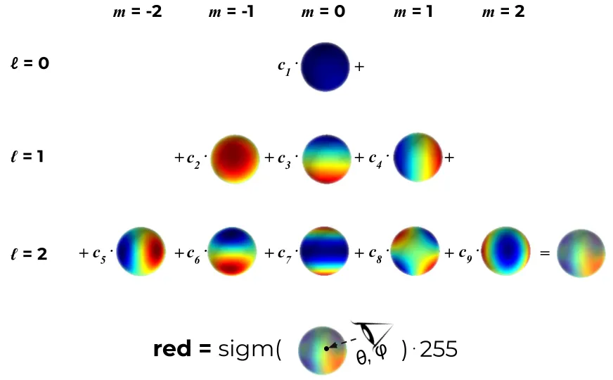
Fig 7. View-dependent colors are comprised of spherical harmonic basic functions. [3].
Controlling Gaussians
Potential Issue #1:
- Areas with missing geometric features(under-reconstruction).
- Regions where Gaussians cover large areas in the scene (over-reconstruction).
Both scenarios result in large view-space positional gradients.
- Intuition: When there is a lack of Gaussians, Gaussians in the neighborhood will want to move toward the under-reconstructed area to improve coverage. When there is a large Gaussian, nearby Gaussians will want to move away from the over-reconstructed region.
Solution: Densification
- Small Gaussians in under-constructed regions: Clone the small Gaussian at the same location and move its clone in the direction of
the positional gradient.
- Increases both the total volume of the system and the number of Gaussians.
- Large Gaussians in regions of high variance: Replace the large Gaussian with 2 new ones and divide
their scale by a factor of 𝜑 = 1.6 (value determined experimentally). Initialize their positions using the original, large Gaussian as a probability density function for sampling.
- Conserves the total volume of the system but increases the number of Gaussians.
Potential Issue #2:
- Floaters that appear close to the input cameras could cause an unjustified increase in Gaussian density.
- Intuition: Floaters could be perceived as over-constructed regions, which the aforementioned algorithm adjusts for through densification.
Solution: Pruning
- Set \(\alpha\) (opacity) close to 0 every 3,000 iterations, effectively pruning the Gaussians.
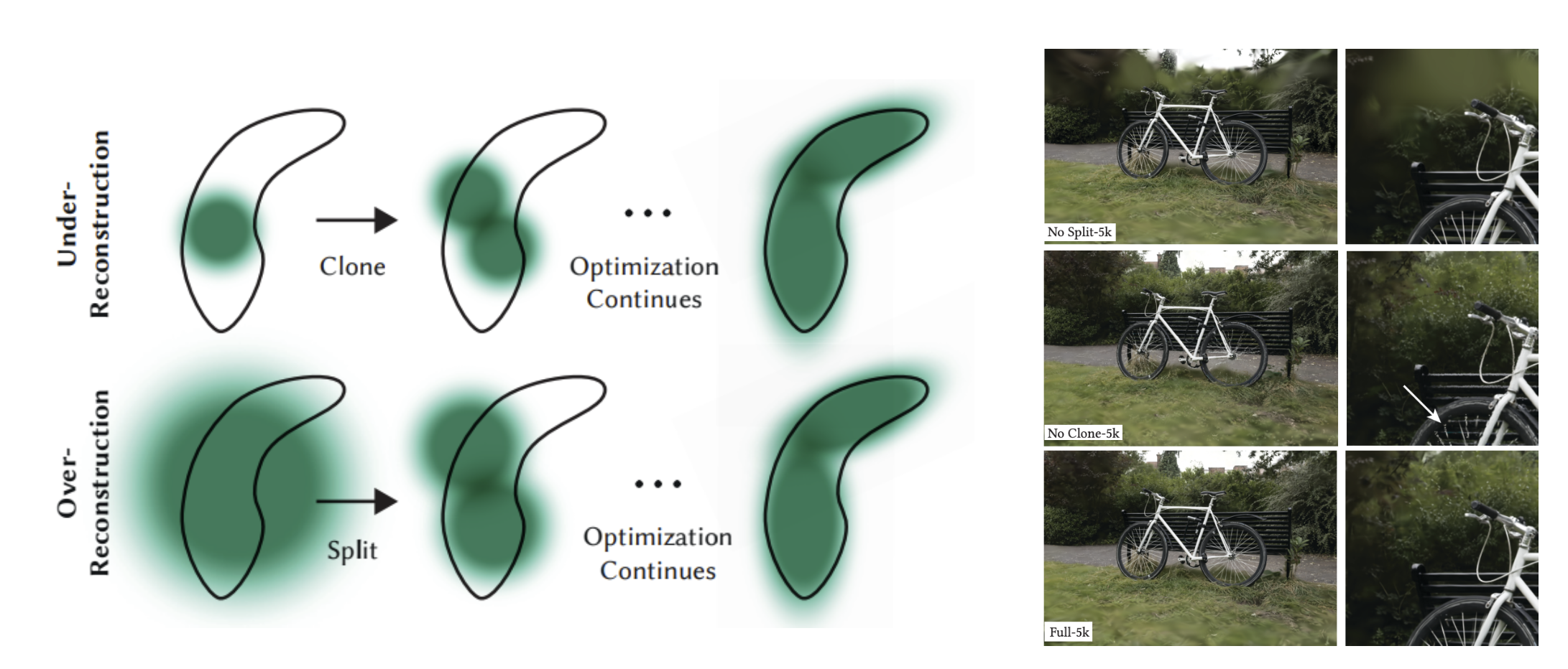
Fig 8. Visualization of densification and pruning of Gaussians [4].
Additional Optimizations:
- Gaussians remain primitives in Euclidean space, meaning they don’t require space compaction, warping, or projection strategies (for distant and large Gaussians).
- Unfortunately, this also leads Gaussian Splatting to be more memory intensive.
Evaluation Metrics
In addition to the aforementioned SSIM, the Peak Signal to Noise Ratio (PSNR) and Learned Perceptual Image Patch Similarity (L-PIPS) metrics are also widely used in the context of novel view synthesis [3].
PSNR is the measure of the ratio between the maximum possible power of a signal and the power of the corrupting noise. For 8-bit images, this is the maximum pixel intensity, \(255\). Less noise results in a higher PSNR value, which is indicative of a higher fidelity reconstruction.
As opposed to calculating pixel-level differences (SSIM and PSNR), L-PIPS measures the distance between two images in a feature space. Typically, the feature maps compared are extracted after passing the original and reconstructed image through a pre-trained deep neural network, making this a learned and adapting metric. Once again, we obtain a similarity score, with a higher value denoting a better quality reconstruction.
Pros and Cons
One of the major advantages of 3D gaussian splatting is its superior rendering efficiency in comparison to NeRFs, while achieving similar if not better performance on multiple metrics. These findings by the original authors are summarized below.
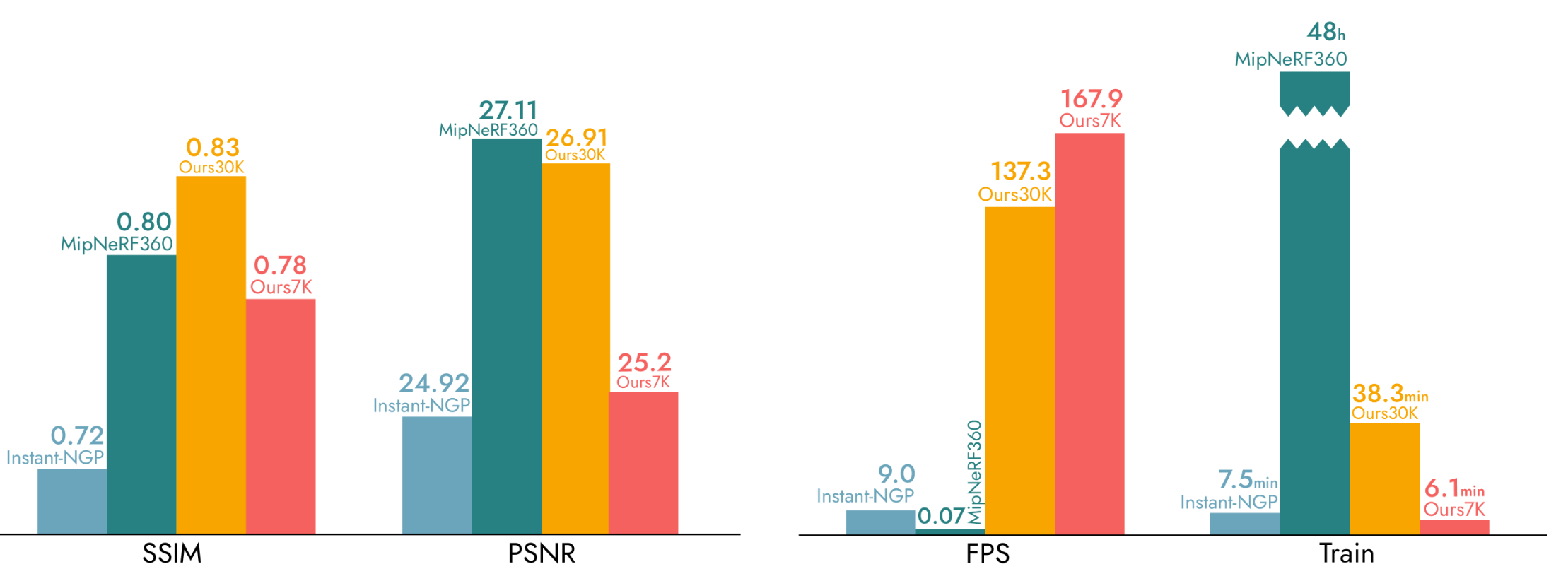
Fig 9. Performance chart for 3D-GS across multiple metrics. [3].
As evident from the charts, the FPS (frames per second) for rendering scenes with a gaussian splat is significantly greater than that of NeRFs. This is largely attributed to the fact that we don’t have to query a neural network for each point. Instead, 3D-GS can directly compute the projected gaussians beforehand and utilize various algorithmic techniques discussed previously to drastically reduce computation time.
We can also see 3D-GS’s strong representational accuracy through the SSIM and PSNR metrics. Through multiple experiments, it’s shown that within a short training period, 3D-GS can match the performance of train-performant methods like InstantNGP and Plenoxels, and on the long-term it can achieve SOTA quality, beating Mip-NeRF360. We can also visually compare the capabilities of these models with a couple examples.

Fig 10. Visual comparison of novel views. [3].
With the bicycle example, we can see that 3D-GS is able to retain high frequency detail, namely with the tire spokes, which is something that even Mip-NeRF360 struggles with. This is reinforced in the latter scene, where it is evident that even for areas further from the camera, gaussian splatting does the best job at preserving high spatial-frequency details.
Another aspect to note is that because our scene representation is defined purely based on gaussians, it allows for more direct manipulation and editing of scenes as seen in following works.
Despite the seemingly boundless amount of benefits, there are definitely some limitations to this approach. One major issue arises from the existence of floating artifacts (especially elongated ones) that may be the result of trivial culling in the rasterization process. In addition, although the rendering speed is much faster, gaussian splatting requires a lot more memory to train due to the millions of gaussians required to accurately render a scene.
Experiments
We ran and tested the original 3D gaussian splatting implementation on a train scene from the Tanks&Temples dataset. As mentioned in the algorithm overview, in order to intialize our gaussian splat, we want to first generate a pointcloud estimate of the 3D scene using Structure from Motion. Because of the heavy time consumption of this process, we utilize the COLMAP results from a public HuggingFace repository [10].
After obtaining this input data, we clone the official GitHub repo from the original authors and run python train.py -s tandt/train where tandt/train was the directory containing the COLMAP results for the train scene. We run the training process for \(30000\) iterations to achieve a decent gaussian splat for visualization. To visualize our gaussian splat on the browser, we run a WebGL tool made by Kevin Kwok [11].
Observations
We noticed many interesting results when visualizing our trained Gaussian Splatting model on the train image. We noticed there was still an issue with large world-space Gaussians, as we can observe large, elliptical blurs clustering around the edges of the original 2D images (sky, ground). While the primary subject of the splat, the train engine, and its nearby objects are relatively well rendered and have few visual artifacts, our model still fails to render to objects less visible in the training images, especially unseen views (including the background). We also notice patchy areas, where it’s clear that there is under-reconstruction and a distinct lack of gaussian to fill the volume, with parts of the mountainous terrain missing.
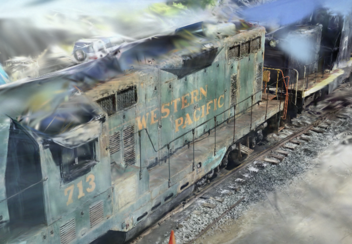
Fig 11. Novel view generated from 3D gaussian splatting.
Conclusion
In this article, we investigated three approaches for novel view synthesis and presented a myriad of strengths and weaknesses. While the field continues to advance, NeRFs and Gaussian Splatting remain the strongest contenders in the field of novel view synthesis. Compared to classical approaches such as light fields, modern methods result in increasingly higher resolution renderings, with similar or less memory and training data required. Among these new techniques, 3D-GS has recently gained recognition for a balance between high fidelity generations and time to generate, able to achieve comparable or superior results to SOTA methods such as NeRFs. In many commerical applications that require real-time rendering such as augmented reality, while having access to limited computational resources and time, 3D-GS may be preferred as opposed to NeRFs.
Future Works
The novel view synthesis problem is currently being heavily researched, and new approaches are being proposed at a frequent rate. As mentioned earlier, the standard 3D-GS method requires storing thousands of gaussians, requiring large amounts of memory. One paper accepted into CVPR 2024 introduces a space-efficient 3D Gaussian Splatting technique, utilizing a similar vector quantization technique in the original light fields paper to compress Gaussian attributes [8]. Through benchmarking, they show their method maintains the quality of 3D-GS while using 25x reduced storage.
Our group is also interested in the application of style transfer in gaussian splatting. Currently, there have been works about applying style transfer to NeRFs to allow for a styled synthesized scene. The challenge, however, of applying a similar concept to 3D-GS is that unlike NeRFs, 3D-GS creates an explicit representation of the scene. As a result, to perform style transfer, we would have to come up with an alternative strategy different than just training a neural network on styling. Some solutions in involve potentially applying style transfer to the scene before the 3D-GS process, but future works could look into applying the style transfer into the splatting pipeline.
Reference
[1] Levoy M, Hanrahan P. “Light Field Rendering. In: Seminal Graphics Papers: Pushing the Boundaries, Volume 2.” 1st ed Association for Computing Machinery; 2023. https://doi.org/10.1145/3596711.3596759
[2] Mildenhall, Ben, et al. “NeRF: Representing Scenes as Neural Radiance Fields for View Synthesis.” In Proceedings ECCV. 2020.
[3] Rubloff, Michael. “What Are the NeRF Metrics?” Radiance Fields, 11 June 2023, https://radiancefields.com/what-are-the-nerf-metrics/.
[4] Kerbl, Bernhard, et al. “3D Gaussian Splatting for Real-Time Radiance Field Rendering.” ACM Transactions on Graphics, presented at SIGGRAPH 2023, Aug. 2023, https://repo-sam.inria.fr/fungraph/3d-gaussian-splatting/3d_gaussian_splatting_low.pdf.
[5] Yurkova, Kate. “A Comprehensive Overview of Gaussian Splatting.” Towards Data Science, 23 December 2023, https://towardsdatascience.com/a-comprehensive-overview-of-gaussian-splatting-e7d570081362.
[6] Ebert, Dylan. “Introduction to 3D Gaussian Splatting.” 2023. https://huggingface.co/blog/gaussian-splatting
[7] Wang, Zhou, et al. “Image Quality Assessment: From Error Visibility to Structural Similarity.” 2004, https://www.cns.nyu.edu/pub/eero/wang03-reprint.pdf.
[8] Joo Chan Lee, Daniel Rho, Xiangyu Sun, Jong Hwan Ko, and Eunbyung Park. “Compact 3D Gaussian Representation for Radiance Field.” arXiv preprint arXiv:2311.13681 (2023) https://arxiv.org/abs/2311.13681
[9] Jeong, Yoonwoo. “NeRF: Representing Scenes as Neural Radiance Fields for View Synthesis.” 29 August 2020, https://towardsdatascience.com/nerf-representing-scenes-as-neural-radiance-fields-for-view-synthesis-ef1e8cebace4.
[10] Duru, Camen. “Gaussian Splatting.” 08 August 2023, https://huggingface.co/camenduru/gaussian-splatting.
[11] Kwok, Kevin. “splat.” 06 January 2024, https://github.com/antimatter15/splat.