Image Inpainting
Image inpainting is the task of reconstructing missing regions in an image, which is important in many computer vision applications. Some of these applications include restoration of damaged artwork, object removal, and image compression.
Web Demo
Before you move onto our report… Watch the video above to see our live web demo of the Partial Convolution paper, which we will discuss shortly! See our source code for more technical details on how we did this.
Introduction
Image inpainting is the task of reconstructing missing regions in an image, which is important in many computer vision applications. Some of these applications include restoration of damaged artwork, object removal, and image compression.
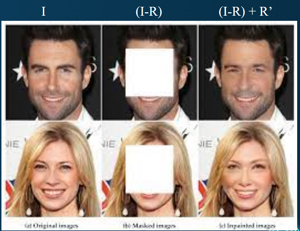
Fig 1. The formalized image inpainting problem.
To formalize the problem of image inpainting, given an image I with a missing region R, the goal is to predict the contents of the missing region R based on the contents of (I-R) and optionally a mask M. For now we can call the outputted region R’.
Most architectures will take in as input (I-R) and a binary mask M indicating which regions need to be inpainted. They will usually then output the inpainted image (I-R) + R’
Datasets/Metrics
Two common datasets that are used are:
- Places2: Over 10 million images spanning more than 400 unique scene categories. Offers a diverse set of backgrounds for inpainting challenges.
- CelebA: More than 200,000 celebrity images, each annotated with 40 attribute labels. Ideal for testing inpainting algorithms focused on human faces.
Performance on these datasets is measured using a variety of metrics, such as the FID for example, which measures the Frechet distance between feature vectors of real images vs. generated images. These feature vectors are obtained by passing images through a layer of the Inception v3 model pre-trained on the ImageNet dataset.
Previous Classical Methods
Many classical methods have been used for Image inpainting, the most notable being patch-based and diffusion-based methods. Patch-based methods focus on finding patches within the image similar to neighboring patches to fill in the missing region. However, these methods are computationally expensive and develop no semantic understanding of the image, which is worrisome when there may be no suitable patches within the image to fill in the missing region.
Diffusion-based methods use mathematical models to transfer information from non-missing parts of the image to the missing regions. The main problems with these methods are that they struggle with recreating missing regions when the image is full of complex textures: diffusion works best when the missing regions have smooth transitions with the rest of the image. Another big problem is that these methods usually lead to blurring at the edge of the missing areas.
Deep-learning based methods have shown to be highly effective at image inpainting due to their ability to learn semantic information from the image. Unlike patch-based methods that rely on an existing patch in the image to serve as a good replacement for the missing regions, deep-learning methods can learn a semantic understanding of the image and recreate the missing region using information it learns from the image and its pre-trained data, usually from ImageNet. In this report, we discuss two recent deep-learning approaches that have built on and improved on past results in the literature for image inpainting, specifically when it comes to inpainting irregular missing regions.
Partial Convolution
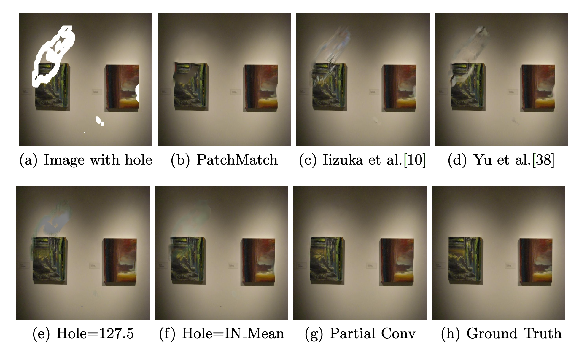
Fig 2. Partial Convolution performs the task better than previous classical (PatchMatch) and deep-learning methods from Iizuka et al. [2] and Yu et. al. [3]
As seen in Figure 2, partial convolutions for image inpainting improved on previous classical implementations, such as PatchMatch [1], which used efficient nearest-neighbor approaches to determine how to fill in the missing regions. Partial convolutions also improved on previous deep learning methods by not requiring initialized values for masked regions. Before, these randomly initialized values previously led to artifacts in the resulting images, such as in Iizuka et. al [2], where they tried post processing techniques of Content Encoder and global and local discriminators, or Yu et. al [3], where instead of post processing they used a refinement network driven by contextual attention layers.
By using a classic U-Net architecture—except replacing convolution layers with partial convolutions—the partial convolution-based model is able to learn semantic information about the image that better fills in missing regions without leading to unwanted artifacts.
The partial convolution operation relies on a binary mask that iteratively updates during training based on previous training steps. Instead of a normal convolution operation, only the valid pixels–the ones that are originally missing–influence the convolution result. During the next iteration, pixels previously non-valid become valid pixels if during any of the convolution operations there was at least one other pixel in the filter that was valid.
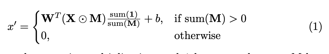
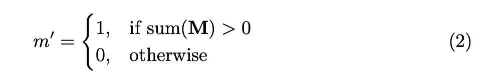
This iterative process of updating the mask m’ allows for an iterative healing process of the image, ensuring that missing regions of the image do not influence convolutions until later convolution layers. Furthermore, the scaling factor, sum(1) / sum(M) helps scale the output value based on the number of unmasked inputs.
For the loss functions, the paper introduces several interesting losses that help achieve good model performance.
Firstly, the per-pixel loss is calculated for both L_hole and L_valid:
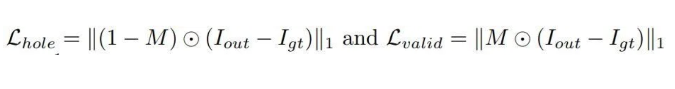
Using the mask M, for both valid and hole pixels, this is simply the L1 loss of the pixel differences between I_out, the output inpainted image of the model, and I_gt, the ground truth image without holes.
In addition to per-pixel losses, the paper also uses the perceptual loss [6]:
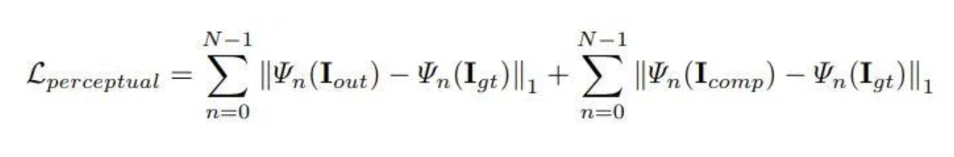
The intuition behind the perceptual loss is that the images generated from the model should lie in a similar latent space to the ground truth images after passing the generated images into a ImageNet-pretrained VGG-16. In the above L_perceptual, Ψ_n represents the activation map of the n-th layer of the VGG model. I_comp represents the result of the image inpainting model, except all of the non-hole pixels are set to their ground-truth value.
Furthermore, the authors define a style loss L_style, which represents how similar in style the model’s inpainted images compare to the ground truth. They do this by applying a Gram matrix transformation to the output of the VGG-16 before taking the L-1 Loss. One intuitive reason for why minimizing the difference between Gram matrices helps to preserve style is that the gram matrix is the result of dot products between flattened feature maps of early layers of the CNN. Thus, each element i,j in the Gram matrix is the dot product between feature map i and feature map j, or in other words, the correlation between the two feature maps.
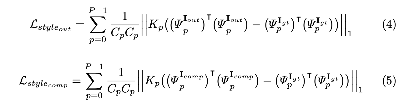
Since these feature maps come from early layers, they generally contain information about shape, texture, and color, so these gram matrices end up containing a lot of information about the texture/style of the picture, which is why the authors end up using L_style to ensure the impainted image is similar in style to the ground truth. Yanghao Li et al. proved that minimizing the difference between Gram matrices of feature maps is the same as minimizing the Maximum Mean Discrepancy (MMD), thereby matching the feature distributions of the generated image and ground truth [7].
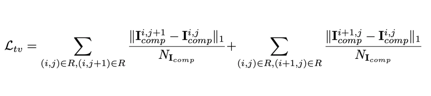
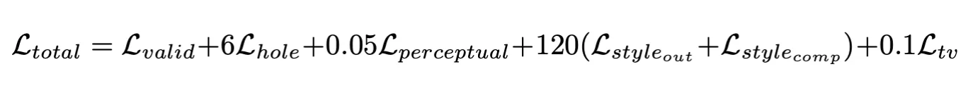
The last unique loss term part of the overall loss term is the total variance loss, loss_TV (TV loss). The TV loss aims to smoothen the re-created regions by penalizing when neighboring pixels in I_comp are significantly different. The overall loss term is a linear combination of the previous loss terms that the researchers found empirically using a hyperparameter search on 100 validation images.
Overall, the approach ends up being significantly more effective for irregular holes or images with more complex textures compared to more classical approaches like PatchMatch [2], since these more classical approaches require neighbors of the image to be able to fill in the hole, which may not be possible for images with complex textures. The perceptual loss combined with the style loss help the partial convolution based architecture to learn semantic information from the picture, allowing it to fill in the missing region in ways that match both the semantic meaning and texture of the image.
Some drawbacks to the partial convolution method is that the model still seems to struggle with very large holes, as do many of the other image inpainting techniques. It is likely that if the model does not have enough information from filled in pixels, it will struggle with recreating a large missing region. The partial convolution method still struggles with sparse structures, such as holes that are part of isolated features, such as this example of a door, where the finer details of the bars are hard for the model to recreate.
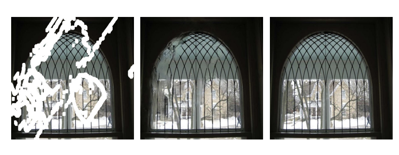
Fig 6. Left: Input to model. Center: Model’s output. Right: Ground truth.
EdgeConnect
EdgeConnect is a Generative Adversarial Network approach to image inpainting [4]. The model has two stages: an edge generation stage and an image completion. As mentioned in the paper, the authors partly came up with this method arising from inspiration from artists who compose their artwork by starting with drawing the edges before filling the spaces inside them later. By combining two generative adversarial networks, the model is able to learn fine-detailed information to fill in missing regions.
The model architecture for EdgeConnect involves many components, including the generator networks, discriminator networks, and several loss functions throughout that help with learning generalizable features to perform the inpainting process.
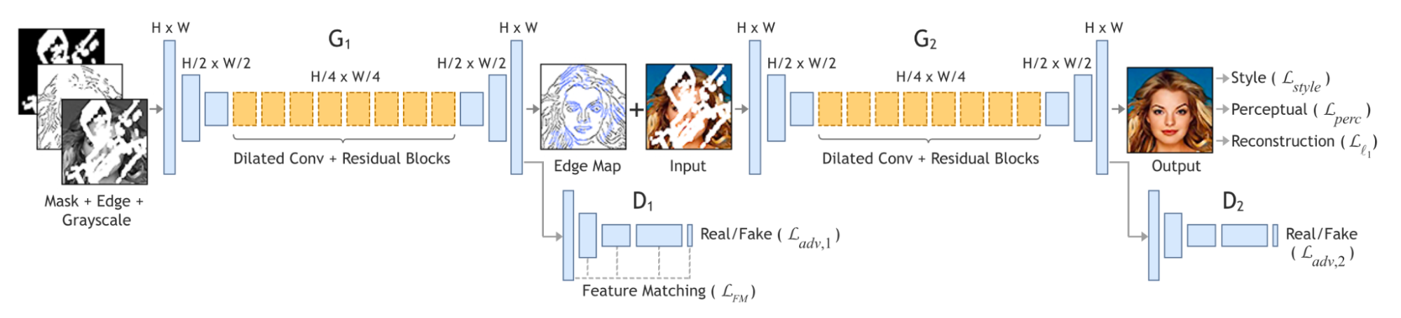
Fig 7. The full model architecture for the EdgeConnect model.
Beginning with the edge generator network, it takes in the masked edge map, which is just the edge map of the image after multiplying with the binary mask M, where 1’s represent missing regions and 0’s represent the background. It also takes in the masked grayscale version of the image. With these three inputs, the generator produces the edge map for the masked region using a U-Net architecture with special dilated convolution and residual blocks.
The ground truth edge maps—since the original images clearly don’t have edge maps—were generated using Canny edge detector [5]. Canny edge detector was used whenever there had to be ground truth labels for the edges in the missing or non-missing regions of the image. Furthermore, the experimenters used both regular and irregular image masks during training. The regular masks were square masks of fixed size, 25% of the image pixels, whereas the irregular masks were augmented versions of these regular masks obtained from the partial convolution paper covered above.
The discriminator then determines if the generated edges are real or fake, and the entire GAN network is trained using two loss functions: an adversarial loss and feature-matching loss.
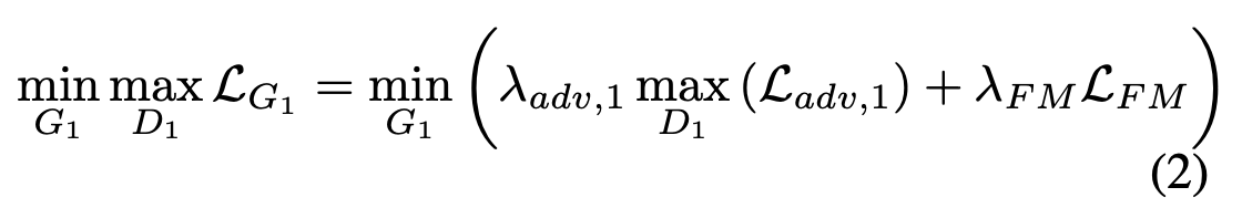
In the total loss formula, λ_adv, 1 and λ_FM are regularization parameters that can be tuned to emphasize either the feature-matching aspect or adversarial part of the overall loss function. The adversarial loss is defined in the paper as the following:
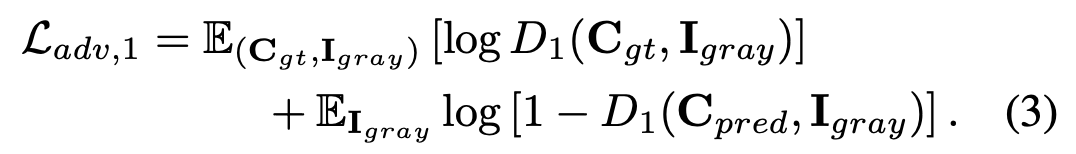
The generator and the discriminator engage in a sort of minimax game, where the generator is trying to fool the discriminator by making the discriminator classify fake images as real ones, whereas the discriminator is trying to not be fooled and correctly classify fake images as fake and real images as real. The first term of the loss function represents cases where the discriminator is passed in real images, and it wants to maximize this value by having D1(x) = 1. For the second term, this corresponds to images that were created by the generator, and so the discriminator wants to maximize this term by having D1(x) = 0, whereas the generator wants D1(x) = 1 because this will minimize the term and overall minimize the entire loss function as seen in equation (2). The network is updated using the alternating gradient updates method.
The feature-matching loss (FM loss) is similar to the aforementioned perceptual loss: it compares the activation maps within the intermediate layers of the discriminator. However, the perceptual loss compared activation maps with those from a pretrained VGG-16, and this does not make sense in this concept of edge generation because the VGG-16 was not trained to produce edge information. The point of the FM loss is to stabilize training by encouraging the generator to produce representations similar to those of the real images.
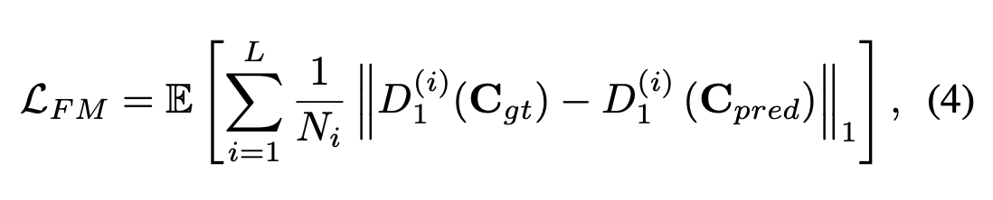
In the FM loss, the L in the summation represents the last convolution layer of the discriminator, N_i is the number of units in the i-th activation layer, and D_1^(i) is the activation in the discriminator’s i-th layer. We can see that the FM loss looks at all activations of the convolution layers for both generated and real images and penalizes the generator for dissimilar representations.
The second part of the overall network, the image completion network, uses as inputs the original color image with missing regions and the composite edge map, which is similar to I_comp from the partial convolution paper—it is the combination of the ground truth edges from the non-missing regions and the generated edges of the network for the missing regions. With these inputs, the image completion network produces a color image, I_pred, with same resolution as the original image.
The image completion network is trained on 4 loss functions: the L1 loss, adversarial loss, perceptual loss, and style loss. The L1 loss, perceptual loss, and style loss are the same as those used in the partial convolution paper, and the adversarial loss is practically identical to the one used for training the edge generator network. Together, these 4 losses allow the generator to learn to fill in missing regions of images so they are similar in style to the ground truth and are overall close in both the pixel-space and latent space of the ground truth images when passed into a VGG network. Using hyperparameters of λ_L1 = 1, λ_(adv, 2) = λ_p = 0.1, and λ_s = 250, their overall loss function for the image completion networks is as follows:

Overall, EdgeConnect is able to produce representations that greatly improve on past classical and deep learning methods, avoiding unwanted artifacts or blurriness. The following figure compares EdgeConnect’s restoration process compared to others like Iizuka et al. [2] and Yu et. al. [3] on a picture with irregular holes, and it is clear it performs quite well at recreating the ground truth image.
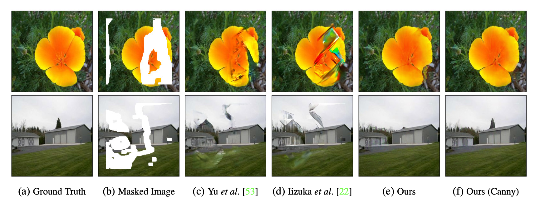
Figure 7. EdgeConnect successfully recreates the missing region compared to past methods like Iizuka et al. [2] and Yu et. al. [3]
Still, as with the partial convolution method, EdgeConnect struggles with recreating large holes or regions with highly complex textures, as seen in Figure 8. The authors believe that with a better edge detector can greatly improve the results of the current model architecture, and this makes sense because edge generation is fundamental to the EdgeConnect model since without good edges, it is likely the model will not be able to produce good final images when these edges are filled in.
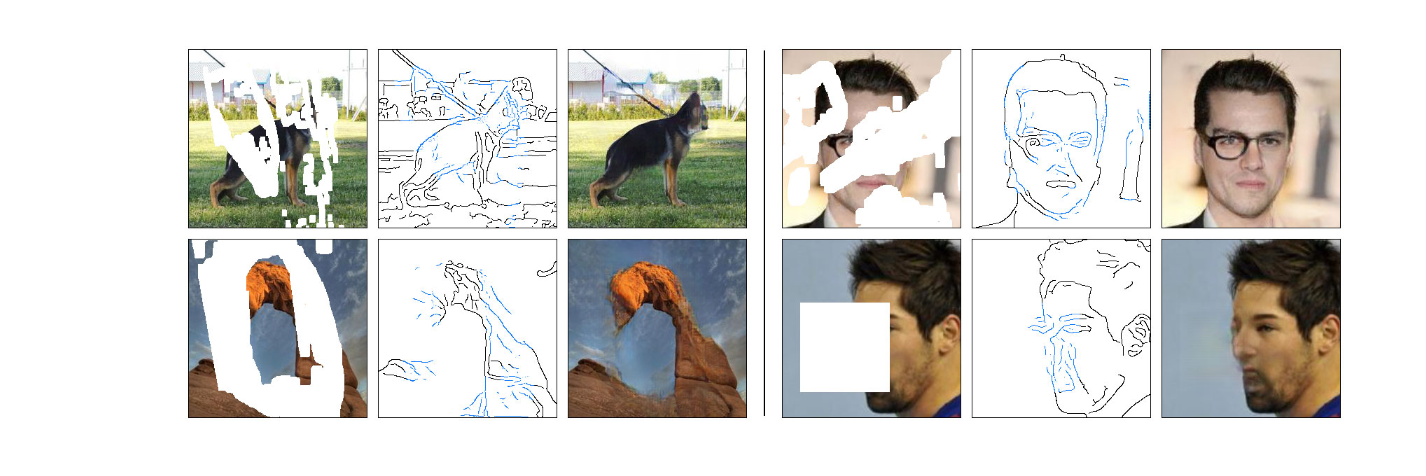
Figure 8. EdgeConnect’s edge generator fails to produce accurate edge information, leading to inaccurate image reconstructions.
Conclusion
In this report, two deep-learning based approaches were discussed: Partial Convolution and EdgeConnect. Both implementations sought to improve on previous solutions that struggled with irregular missing regions in particular. Partial Convolution was a novel way to iteratively heal the missing region and avoid using randomly initialized values for these missing regions that previously caused unwanted artifacts in other methods like Iizuka et al. [2] and Yu et. al. [3]. EdgeConnect used two generative adversarial networks, one generating edges and the other generating the finished image. By harnessing the Canny Edge Detector to generate training labels for edge generation, the generator and discriminator networks work together to build a model that performs the image inpainting problem better than other past classical and deep learning methods.
However, both methods are still not perfect: they struggle with large holes or highly complex texture patterns. It is likely that future work can develop on these two papers to produce deep learning methods that are even more effective at recreating missing regions with complex textures or incredibly large holes. Such an improvement will likely need to stem from even better semantic understandings of images, so that even with limited valid pixels, one can recreate the entire image.
Works Cited
[1] Barnes, C., Shechtman, E., Finkelstein, A., Goldman, D.B.: Patchmatch: A ran- domized correspondence algorithm for structural image editing. ACM Transactions on Graphics-TOG 28(3), 24 (2009)
[2] Iizuka, S., Simo-Serra, E., Ishikawa, H.: Globally and locally consistent image com- pletion. ACM Transactions on Graphics (TOG) 36(4), 107 (2017)
[3] Yu, J.,Lin, Z.,Yang, J.,Shen, X.,Lu, X.,Huang, T.S.: Generative image inpainting with contextual attention. arXiv preprint arXiv:1801.07892 (2018)
[4] Nazeri, Kamyar, et al. “Edgeconnect: Generative image inpainting with adversarial edge learning.” arXiv preprint arXiv:1901.00212 (2019).
[5] Canny, John. “A computational approach to edge detection.” IEEE Transactions on pattern analysis and machine intelligence 6 (1986): 679-698.
[6] Gatys, L.A., Ecker, A.S., Bethge, M.: A neural algorithm of artistic style. arXiv preprint arXiv:1508.06576 (2015)
[7] Li, Yanghao, et al. Demystifying Neural Style Transfer.