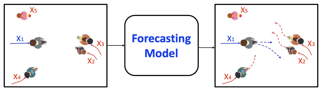
Trajectory Prediction
Estimating the future positions of people or objects (agents) is a crucial capability that can serve diverse applications. These include self-driving cars, as being pursued by Waymo and Tesla, to Hawkeye that can determine an out or not call in tennis, to analyzing crowd behavior to ensure no human-crush occurs. Knowing the past, present, and most importantly, future trajectory of agents is clearly an important tool.
- Introduction to Trajectory Prediction
- Papers and Approaches
- Social LSTMs
- Social GANs
- Comparing Social LSTM and Social GAN
- VectorNet
Introduction to Trajectory Prediction
Estimating the future positions of people or objects (agents) is a crucial capability that can serve diverse applications. These include self-driving cars, as being pursued by Waymo and Tesla, to Hawkeye that can determine an out or not call in tennis, to analyzing crowd behavior to ensure no human-crush occurs. Knowing the past, present, and most importantly, future trajectory of agents is clearly an important tool. The following approaches all try to solve the central problem: given the current state, and other environment variables, where would the agent be in the next state.
Papers and Approaches
Social LSTMs
Social LSTM: Human Trajectory Prediction in Crowded Spaces [1]
Humans have the ability to “read” one another, predicting each other’s general motions, each obeying a set of untold rules that help us predict the motion of other humans. However, trying to predict this motion with machines has proven to be a difficult task. Previous methods have either used functions to predict behavior or only consider other people in close proximity.
Social LSTMs tackle the problem of trajectory prediction, more specifically pedestrian trajectories, and allow for anticipating more distant interactions.
Social LSTM Architecture
Social LSTMs base themselves on the traditional LSTM architecture, which has proven to be very useful for sequence prediction tasks such as caption generation, translation, video translation, and more. In their specific model, the authors of Social LSTM introduce a few key ideas. Firstly, each trajectory is represented by its own LSTM model. Secondly, the LSTMs are linked to each other via a special layer called a social pooling layer.
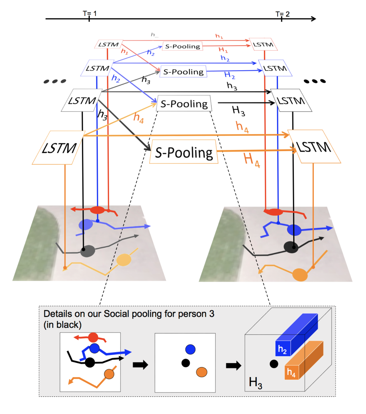
This social pooling layer is based on human intuition. Individuals usually make decisions about their path based on the motion of neighboring people and other surrounding objects. At each timestep, each LSTM cell receives pooled hidden state information from neighboring LSTM cells. These “Social hidden-state” tensors are encoded with positional information. With this, we can predict a new position for each trajectory.
This method has proven effective for groups of individuals, not just predicting individuals.
Social GANs
Social GAN: Socially Acceptable Trajectories with Generative Adversarial Networks
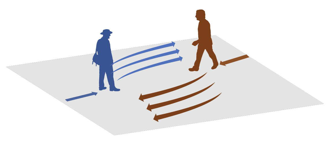
Pedestrians moving towards one another with socially-acceptable predictions. [2]
Introduction
Human motion is inherently ‘multi-modal’: given any position, we have many ‘socially plausible’ methods of maneuvering throughout space to get to our destination. This suggests modeling a recurrent sequence to make predictions on future behavior and pooling information across various agents that impact possible suggested movements. Previous methods, RNN-based architectures and traditionally used methods based on specialized features (i.e. physics-based approaches) suffered from certain primary limitations: using only a neighborhood of agents to compute due to being unable to model interactions between all agents in a computationally efficient manner (1) and only being able to learn ‘average behavior’ instead of generally acceptable and more likely behaviors based on a history of movements at a given time step (2).
Social GAN Architecture
This following proposed architecture addresses these limitations by employing Generative Adversarial Networks which have empirically been able to overcome intractable probabilistic computations and further projections of behaviors. Instead of generating images, as has been commonly employed in the past, the architecture proposes to generate multiple trajectories given a history where a generator creates candidates and the discriminator evaluates them, pushing the generator to learn ‘good behaviors’ that can fool the discriminator (to generate ‘socially acceptable motion trajectories’) in a crowded environment with numerous agents.
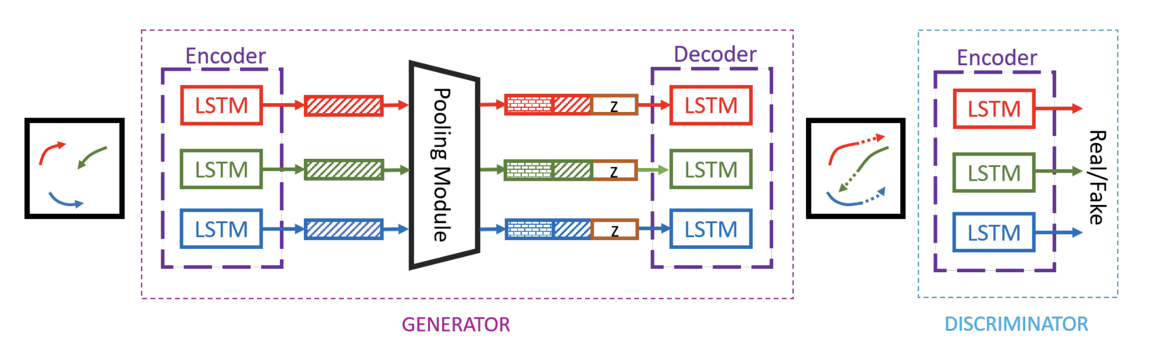
Encoder-decoder structure connecting LSTM cells of the Social-GAN architecture with both generator and discriminator. [2]
The model: an RNN Encoder-Decoder generator and RNN-based encoder discriminator with variety loss to encourage the generator to explore various plausible paths while being consistent with provided inputs, combined with global pooling to encode information with respect to all agents in a given scene. In the provided figure, there are several key components, the initial generator (\(G\)), pooling module, and discriminator (\(D\)). \(G\) takes in previous trajectories \(X_i\) and encodes the history of individual \(i\) as \(H_i^t\) where \(t\) indicates the current time. The pooling module takes input the hidden state of the currently observed hidden state for each individual and outputs a pooled vector \(P_i\) for each person. The decoder then produces the future trajectory conditioned on the latest observed hidden state \(H_i^{t_{obs}}\) and \(P_i\). \(D\) takes in as input whether or not the trajectory is real or fake and classifies them as socially acceptable or not. This allows for the generator to converge on a predicted series of probabilities for given agents within a scene. Given all agents in a scene \(X = X_1, X_2, …, X_n\), the goal is to predict all future trajectories simultaneously such that the input trajectory of person i is defined as \(X_i = (x_i^t, y_i^t)\) for a \(t=1,...t_{obs}\) and the future trajectory is defined similarly with \(Y_i = (x_i^t, y_i^t)\) from time steps \(t=t_{obs} + 1,...,t_{pred}\).
GANs
The generative adversarial network functions with two neural networks trained in complete opposition where generative model \(G\) attempts to use the probabilistic data distribution to ‘fool’ the discriminator and discriminative model \(D\) that estimates the probability that a provided sample was from \(G\) versus the training set. \(G\) inputs a latent variable, \(z\), and outputs a generated sample \(G(z)\); \(D\) takes in a sample \(x\) and outputs whether or not the input belongs to the data set or not. Thus we have the following ‘min-max objective’:
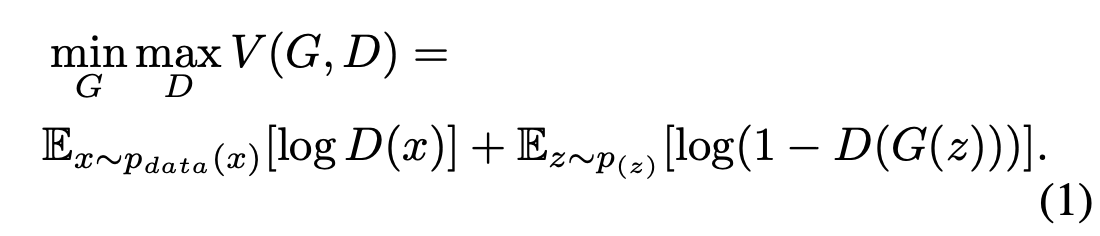
GAN optimization formula. [2]
where we maximize the capability of the discriminator and minimize \(G\) to become close to generative distribution of the data such that the discriminator cannot tell the difference.
Socially-Aware GANs
The model consists of the aforementioned 3 key components: Generator (\(G\)), Pooling Module (\(PM\)) and Discriminator (\(D\)); \(G\) takes inputs of agents \(X_i\) and outputs predicted trajectories of said agents \(\hat{Y}_i\). \(D\) takes as input the entire sequence from the input movement trajectory and future predictions (\(X_i\), \(\hat{Y}_i\), respectively) and classifies whether or not each provided sequence/trajectory prediction pair is fake or real.
With the generator, using \(\phi(\cdot)\) as a single layer MLP with ReLU non-linear activation, \(W_{ee}\) as the embedding weight, \(W_{encoder}\) as the shared embedding weight between all individuals, and the given locational input \(x_i^t, y_i^t\), we obtain the following recurrence for the embeddings of each agent at time t for the LSTM cell of the encoder:
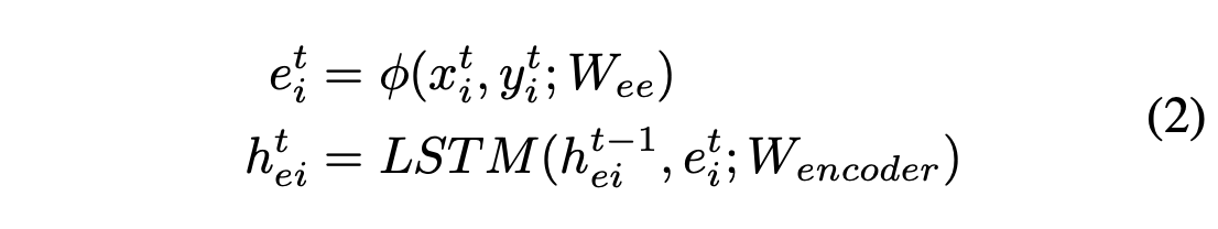
Encoder initialization. [2]
However, one LSTM per person fails to capture the understanding of inter-agent interactions, so this is modeled via the Pooling Module such that each hidden state for all agents interact, giving a pooled hidden state \(P_i\) for each person i.
To produce future scenarios with respect to the past, the generation of new output requires a conditional for the decoder initialization:
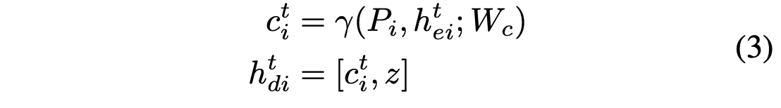
Decoder initialization. [2]
where \(\gamma(\cdot)\) is a fully-connected layer with ReLU activation and \(W_c\) as the weight embedding.
After the given encoder and decoder initialization, we obtain the predictions as follows:
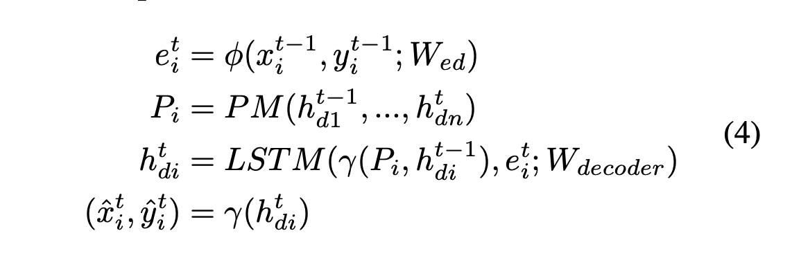
Final predictions of the model. [2]
The discriminator ultimately consists of a separate encoder which takes as input some real or generated data and classifies them accordingly. Based on the encoder’s last hidden state, the model uses an additional fully-connected layer to generate a classification score. This ideally teaches subtle social interaction rules and classifies trajectories that aren’t acceptable as ‘fake’, using L2 loss on top of adversarial loss to indicate how ‘far’ generated samples are from the ideal data distribution. To further encourage diverse samples on trajectory prediction (in the case of being able to move in multiple directions to mimic humans’ multi-modal movement capability), the authors employed a variety loss function which selected the best of \(k\) generated output predictions by randomly sampling the latent space!
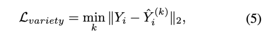
L-variety loss optimization for best trajectory. [2]
This loss considers only the best trajectory, pushing the network to cover the space that best conforms to the past trajectory and provides high probabilistic predictions in realistic directions.
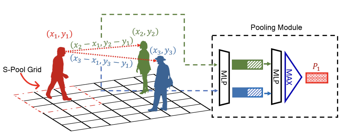
Social Pooling (red-grid) vs. Social GAN Pooling Mechanism (distance metric comparison). [2]
Discussion
Using the LSTMs, the authors were able to determine the hidden states with respect to each individual agent, but this additionally requires a mechanism to share information across LSTMs (i.e. between individuals). This is directly enabled with the pooling module in computing a resultant hidden state using the hidden states of all LSTMs for each agent; the module handles primary issues when scaling to variable numbers of people across a large crowd and handling human-to-human interactions that may be significantly more scarce environment (where agents further away may still impact one another, albeit to a lesser degree). With other social pooling mechanisms, they fundamentally work by employing a grid-based pooling scheme which fails to capture global extent as it only considers within the grid whereas the Pooling Module computes relative positions between each agent and all other agents which are concatenated with the person’s hidden state and processed independently via MLP. This allows the final pooled vector \(P_i\) to summarize all the information a person needs to make a decision to ‘move’.
When removing the pooling, we observe that agents fail to consider the paths of others, which in turn may result in convergent pathways (which are realistically infeasible when considering walking scenarios). Pooling via relative distance enforces a global understanding of other agents and what is technically feasible with respect to the current state of agents and the ‘conformity to social norms’ and practices when referring to movement. Observe the following image where we have agents without the pooling mechanism (SGAN) versus agents with the pooling mechanism (SGAN-P).
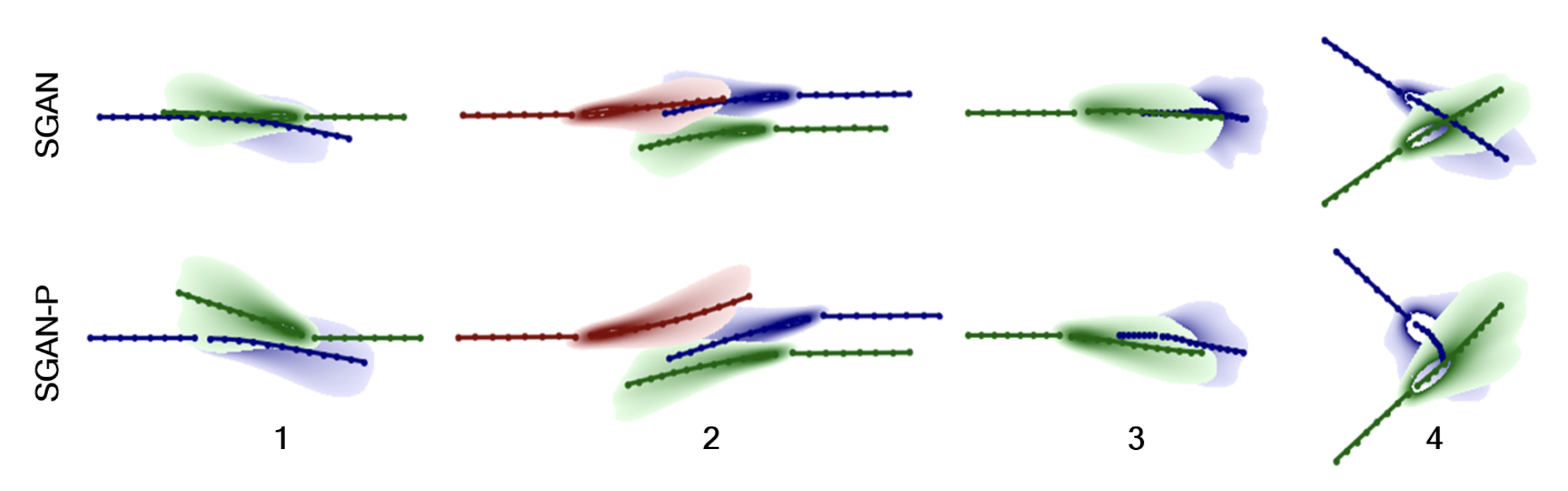
SGAN vs. SGAN-P (without pooling and with pooling mechanism integrated into architecture prediction performance comparison) [2]
This directly mimics human behavior in representing those tending towards the same direction, depicting human tendency to vary pace in order to avoid collision (scenario 3) and even yield right-of-way (scenario 4). And, this represents the tendency to react to incoming movement as well (particularly in group behavior). Using information with respect to the pace of the person and the particular direction of movement (gathered from the initial time-steps), the paper observed different ‘reactions’ of predictions to the movement of crowds.
Another key observation was made relative to the latent space: in understanding the latent space \(z\), particular directions within the latent space were directly associated with the direction and speed of the agents that served as the future predictions in upcoming time steps.
Overall, this methodology proposes a novel solution to generating predictions based on global interactions via a relative-distance pooling method, allowing the network to learn social norms of agent-movement by training against a discriminator. In directly imposing a variety loss with said pooling layers, this allowed training of a network that could produce multiple viable probabilistic solutions to trajectory predictions given diverse samples.
Comparing Social LSTM and Social GAN
Social LSTM and Social GAN are two methods of trajectory prediction that focus on socially accetable trajectories. They can both be applied to street pedestrian-esque problems, and thus can be effectively compared using this kind of scenario.
We decided to evaluate and compare Social LSTM and Social GAN using the TrajNet++ Framework that is based on [3]. Setup of all framework was completed using the following resource. This platform uses Python, specifically PyTorch for model implementations and torch-geometric for data representation and loading.
Dataset
Optical Reciprocal Collision Avoidance (ORCA) is a process for generating collision-free motion with agents. TrajNet++ is compatible with the RVO2 Library implementation of ORCA, and we use this to generate data of agent trajectories. Note that these trajectories are most similar to pedestrian movement and are not restricted to roads like cars are. Our data includes 1000 scenarios of 5 pedestrians at a circular crossing. The simulator generates ground truths of the trajectories of the pedestrians for each scenario. A train, test, validation split is performed.
Using the TrajNet++ framework, data could be generated using python and the command line. The call we used to generate was as follows:
python -m trajnetdataset.controlled_data --simulator 'orca' --num_ped 5 --num_scenes 1000
We then process the data scenes to include scenes where interactions happen:
python -m trajnetdataset.convert --linear_threshold 0.3 --acceptance 0 0 1.0 0 --synthetic
An example of an interaction between the agents is shown here:
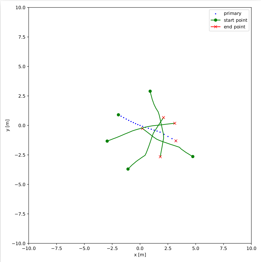
Paths for 5 different agents.
Model Training
Models were TrajNet++ implementation of Social LSTM and Social GAN based on the papers. Their implementations can be found here.
The following was used to initialize the baseline Social LSTM model and train it:
python -m trajnetbaselines.lstm.trainer --type social --augment --n 16 --embedding_arch two_layer --layer_dims 1024
The following was used to initialize the baseline Social GAN model and train it:
python -m trajnetbaselines.sgan.trainer --type directional --augment
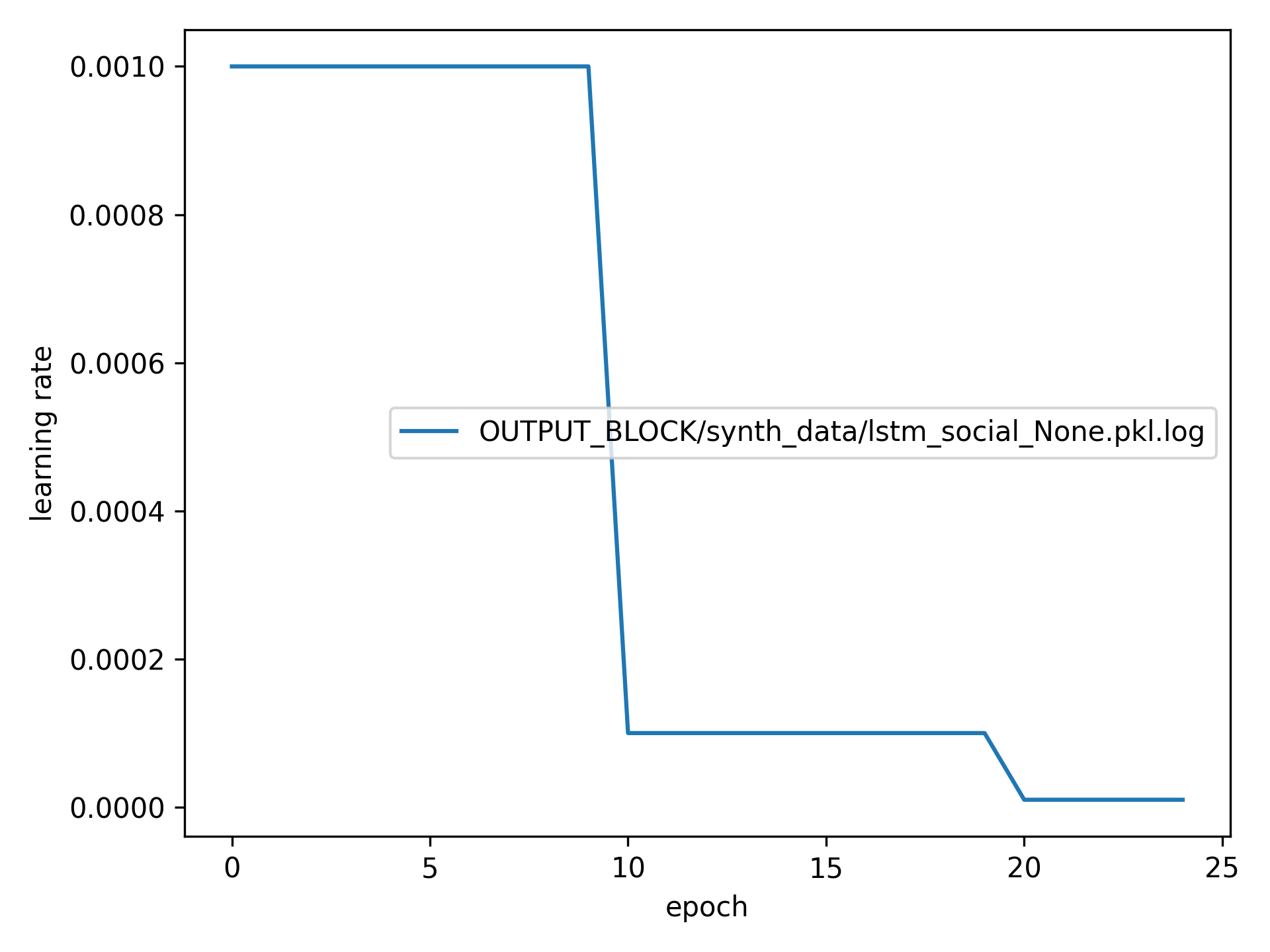
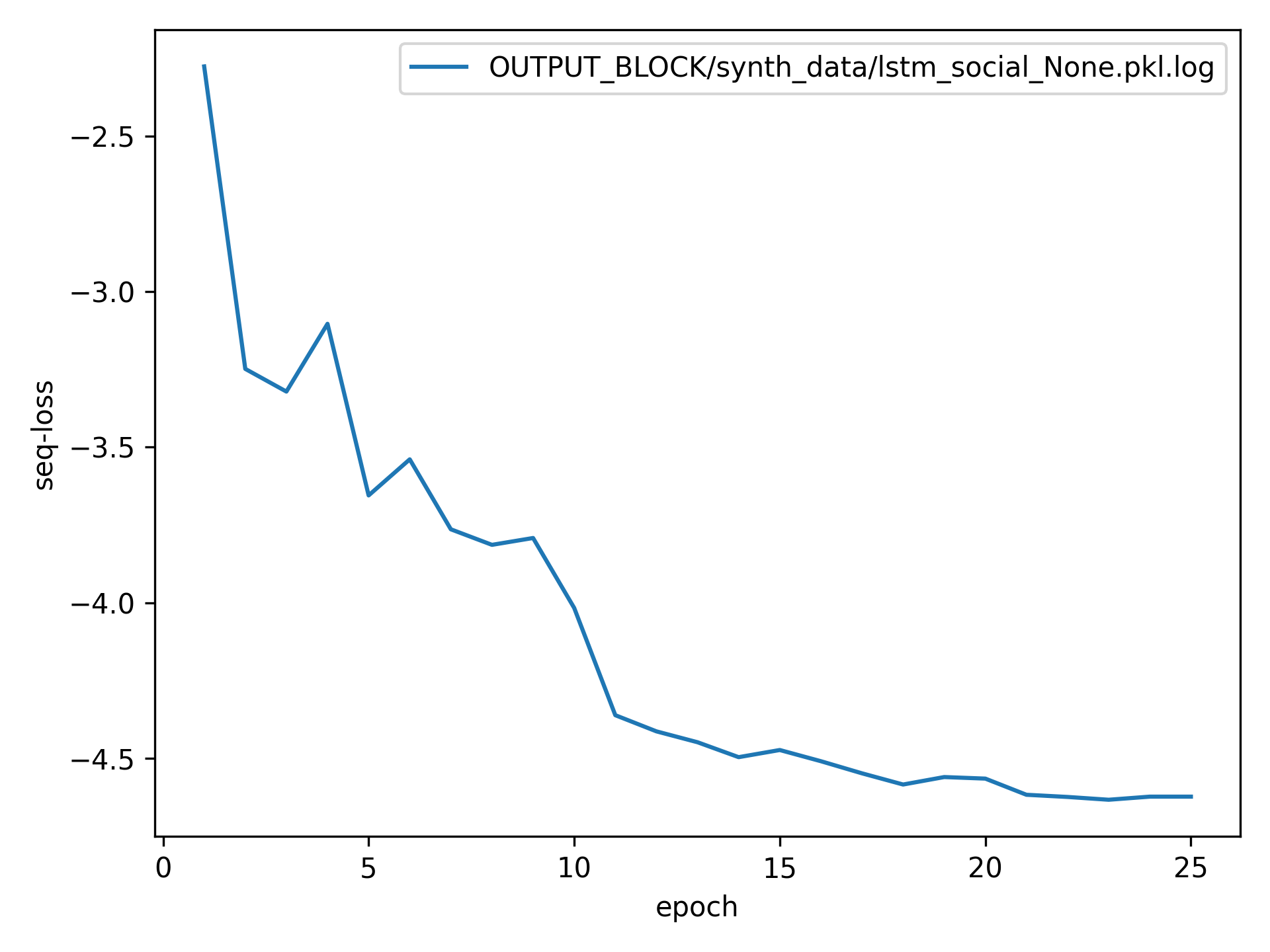
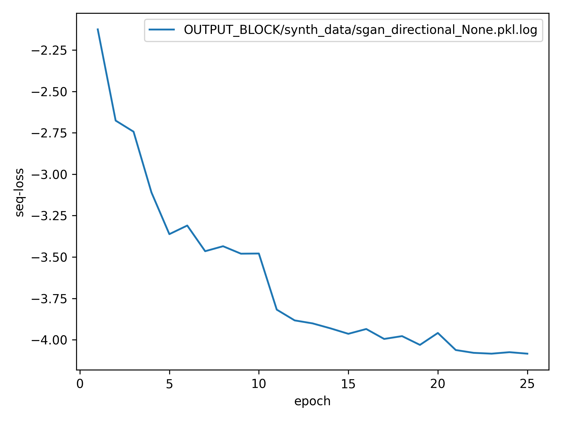
All models were trained for 25 epochs using PyTorch Adam optimizer with
lr=1e-3,weight_decay=1e-4. Learning rate was annealed using the following schedule:
Training Loss Curves
Social LSTM
Social GAN
Results
Evaluation
TrajNet++ has ample evaluation scripts that capture relevant trajectory prediction metrics. The following was used to evaluate the trained models:
python -m trajnetbaselines.lstm.trajnet_evaluator --output OUTPUT_BLOCK/synth_data/lstm_social_None.pkl --path synth_data
python -m trajnetbaselines.sgan.trajnet_evaluator --output OUTPUT_BLOCK/synth_data/sgan_directional_None.pkl --path synth_data
Metrics
Average Displacement Error (ADE): Average L2 distance between the ground truth and prediction of the primary pedestrian over all predicted time steps. Lower is better.
Final Displacement Error (FDE): The L2 distance between the final ground truth coordinates and the final prediction coordinates of the primary pedestrian. Lower is better
Prediction Collision (Col-I): Calculates the percentage of collisions of primary pedestrian with neighbouring pedestrians in the scene. The model prediction of neighbouring pedestrians is used to check the occurrence of collisions. Lower is better.
Ground Truth Collision (Col-II): Calculates the percentage of collisions of primary pedestrian with neighbouring pedestrians in the scene. The ground truth of neighbouring pedestrians is used to check the occurrence of collisions. Lower is better.
Social LSTM

Social GAN

Discussion
Based on the results, we can observe that in these scenarios, the Social LSTM had lower displacement errors for the final predicted trajectories. However, the Social GAN was able to better decrease the occurence of unwanted collisions in accordance with the ground truth (Col-II). The former can be attributed to the generational nature of the GAN not modeling the data as effectively as the LSTM. The latter could be a result of the newer and more complex GAN method being able to handle socially-acceptable trajectories and avoid collisions better.
VectorNet
Introduction
 TrajNet++ benchmark [5]
There are more real world applications for human trajectory forecasting including evacuation analysis, more efficient public transportation, to how crowds behave during chaotic events. Early approaches to this used handcrafted representations based on domain knowledge to predict where people (agents) in a crowd would go. However, social interactions in the crows are diverse and subtle, making these predictions difficult to capture manually. Due to the recent advantages of deep learning - large models are able to accurately predict and outperform handcrafted approaches. VectorNet by Waymo, a self-driving car company backed by Alphabet, is a state-of-the-art deep learning model for trajectory prediction. Its main novel advantages include using vector representations to model spatial agent interactions and employing deep sets architecture to reason about interacting agents. To test the performance of Vector Net, this group uses TrajNet++, a large-scale benchmark tailored for evaluating interaction forecasting.
Architecture
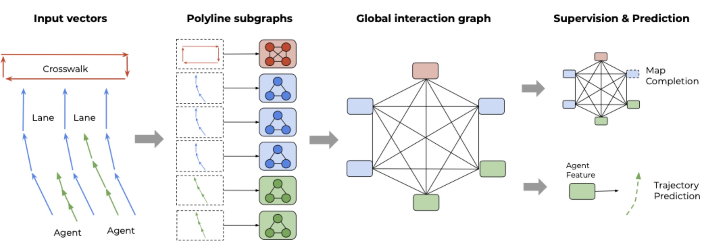 Overall architecture of VectorNet [4]
The architecture of VectorNet has two primary novel strengths. The first being its use of vectors to encode data, whether it be agents, lanes, crosswalks, etc. Vector representation naturally captures the spatial relationships and geometry between agents, which is crucial information about interactions in trajectory prediction tasks. The vector representation also allows for the second main advantage of vector net, GNNs. Conventional neural networks employ a layer-wise architecture, where each layer performs linear transformations followed by non-linear activations to learn relevant patterns from the input data. However, graph neural networks (GNNs) adopt a distinct approach by utilizing neighborhood-based aggregations to generate representations that evolve over iterations. The primary advantage of GNNs lies in their ability to handle tasks that are beyond the scope of traditional Convolutional Neural Networks (CNNs). While CNNs excel at tasks such as object detection, image classification, and pattern recognition, they achieve this through the use of convolutional layers and pooling operations tailored for grid-structured data.
There are two fundamental limitations that hinder the application of CNNs to graph-structured data: 1. Computational Complexity: Applying CNNs to graph data is computationally challenging due to the arbitrary and intricate topology of graphs, which lack the spatial locality inherent in grid-like structures. Additionally, the absence of a fixed node ordering further complicates the utilization of CNNs. 2. Loss of Relational Information: When graph data is projected onto a grid or image representation, valuable information regarding the depth and distance relationships between key entities is lost. This projection process effectively discards the rich relational structure inherent in graph data.
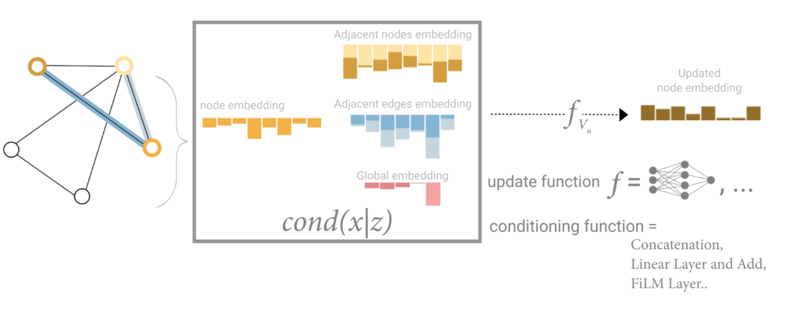 Training VectorNet and retrieving the node/edge embeddings to update weightings for next layer. [4]
Convolutional Neural Networks have demonstrated remarkable success in tackling problems where the underlying data representation exhibits a grid-like structure, such as image classification. These architectures leverage their learnable filters efficiently by applying them to all input positions, thereby reusing local patterns. However, many compelling tasks involve data that cannot be represented in a grid-like format and instead resides in an irregular domain. Examples of such data include 3D meshes, social networks, telecommunication networks, biological networks, and brain connectomes, all of which can be naturally represented as graphs. In GNNs, nodes embed information with regards to an object or entity. This could include positional data or attributes of the object. Edges could represent the relationship between a node and how embeddings update.
For the vector net paper, they set \(v_i = [d_i^s, d_i^e, a_i, j]\). Where each polyline P with nodes \(\{v_1, v_2, …, v_P\}\) defines our subgraph GNN layer as:
\(v_i^{l+1} = \phi_{rel} (g_{enc}(v_i^{(l)}), \phi_{agg}(\{g_{enc}(v_i^{(l)})\}))\),
where \(\phi_{agg}(.)\) is max-pooling, \(\phi_{rel}(.)\) is concatenation. A few other primary equations that Vector Net uses is its loss function: \(L = L_{traj} + \alpha * L_{node}\) Where \(L_{traj}\) is NLL for trajectory prediction, \(L_{node}\) is loss from graph completion task, and \(\alpha\) is the scaling factor. Metrics that can evaluate its performance is the average displacement error (ADE), and the displacement error at t, or the displacement error in meters at time \(t = 1, 2, 3\)
Reference
Please make sure to cite properly in your work, for example:
[1] A. Alahi, K. Goel, V. Ramanathan, A. Robicquet, L. Fei-Fei and S. Savarese, “Social LSTM: Human Trajectory Prediction in Crowded Spaces,” 2016 IEEE Conference on Computer Vision and Pattern Recognition (CVPR), Las Vegas, NV, USA, 2016, pp. 961-971, doi: 10.1109/CVPR.2016.110.
[2] Gupta, A., Johnson, J., Fei-Fei, L., Savarese, S., & Alahi, A. (2018). Social GAN: Socially Acceptable Trajectories with Generative Adversarial Networks (Version 1). arXiv. https://doi.org/10.48550/ARXIV.1803.10892
[3] Kothari, P., Kreiss, S., & Alahi, A. (2020). Human Trajectory Forecasting in Crowds: A Deep Learning Perspective (Version 3). arXiv. https://doi.org/10.48550/ARXIV.2007.03639
[4] J. Gao et al., “VectorNet: Encoding HD Maps and Agent Dynamics From Vectorized Representation,” 2020 IEEE/CVF Conference on Computer Vision and Pattern Recognition (CVPR), Seattle, WA, USA, 2020, pp. 11522-11530, doi: 10.1109/CVPR42600.2020.01154.
[5] P. Kothari, S. Kreiss and A. Alahi, “Human Trajectory Forecasting in Crowds: A Deep Learning Perspective,” in IEEE Transactions on Intelligent Transportation Systems, vol. 23, no. 7, pp. 7386-7400, July 2022, doi: 10.1109/TITS.2021.3069362.