Image Style Translation
Image style translation is the process of converting an image from one style to another. We will explore two deep learning approaches to image style translation: CycleGAN and Stable Diffusion, and compare their performance on the task of converting realistic images to Monet-style paintings.
- Introduction
- Image-to-image translation
- CycleGAN
- Stable Diffusion
- Image Captioning with Transformers
- Experimentation: Approaching Realistic Image to Monet-style Painting
- Discussion
- Reference
Introduction
Style transfer takes the visual style of one image or a subset of image and applying it to the content of another, which makes the synthesis of images that combine the aesthetics of one style with the semantic content of another image. More generally, style transfer aims to translate one image into another in a meaningful way, and deep learning becomes the dominant approach to this problem. We would like to examine style transfer in the context of image-to-image translation. In this paper, we take an in-depth look at two popular deep learning approaches for style translation: CycleGAN and Stable Diffusion, in which we will discuss the high level functionality of each model, how it works, how to train it, and potential limitations. We also experiment with CycleGAN and finetuned Stable Diffusion model, comparing their performance on the task of translating an realistic image to Monet style.
Image-to-image translation
The goal of image-to-image translation is learning a mapping between input image and the output image. The dataset used for this problem is typically two sets of images we want to learn the mapping between. These datasets come in the form of
- Paired: the dataset is tuples of image in set 1 and corresponding image in set 2
- Unpaired: the dataset just has two sets of images without 1-to-1 correspondence.
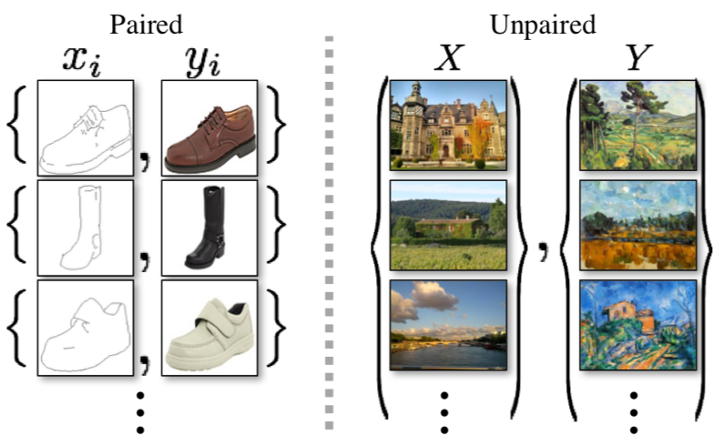 Fig 1. Illustration of unpaired vs paired dataset [5].
Paired datasets are easier to train on, but they maybe hard to collect, especially in style transfer (e.g. cartoon characters may not have good corresponding realistic representations). Thus, we need methods to effectively train on unpaired datasets.
CycleGAN
Generative adversarial network (GAN) are generative deep learning frameworks that rely on a generator \(G\) and a discriminator \(D\). Cycle GAN builds on GAN by introducing cycle consistency (similar to language translation, where a sentence in English when translated to German then translated back should be the same as English).
-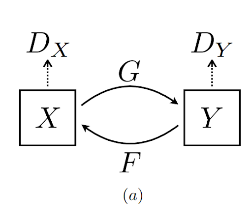 Fig 2. Illustration of Cycle GAN [4].
The goal of CycleGAN is to learn a mapping between two image styles $X$ and $Y$. So if we have preserve cycle consistency, the idea is that our translated image will preserve most of its semantics besides the style change.
-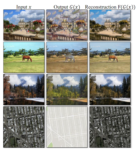 Fig 3. Illustration of Cycle Consistency [4].
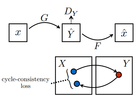
To preserve cycle consistency, we want to make sure when our network translates an image, we can translate it back to get a image similar to the original image. In order to do this, we train two GANs together, Gan 1 \((G, D_Y)\) translating from style \(X\) to style \(Y\). Gan 2 \((F, D_X)\) translating from style \(Y\) to style \(X\). We additionally introduce a normalization term (the cycle consistency loss) on the input image \(I\) and the \(F(G(I))\), the input image translated twice.
| X-Y-X Cycle | Y-X-Y Cycle |
|---|---|
 |
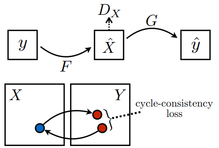 |
Fig 4. Illustration of Cycle Consistency Loss [5].
Now, in the actual style transfer process, we can use \(G\) to translate from style \(X\) to style \(Y\), and \(F\) to translate from style \(Y\) to style \(X\), and disregard the discriminators.
Architecture
The generators \(G\) and \(F\) can be any architecture that can map an image from one domain to another. The implementation provided by the CycleGAN paper uses either U-Net (see [4]) or Resnet-based generator (6 or 9 Resnet blocks combined with downsampling/upsampling operations). The discriminators \(D_X\) and \(D_Y\) are either 70x70 PatchGANs, which classify whether 70x70 overlapping image patches are real or fake, or 1x1 PixelGAN, which classifies whether each pixel is real or fake.
Detailed implementation of Resnet-based generator:
"""
Parameters:
    input_nc (int)      -- the number of channels in input images
    output_nc (int)     -- the number of channels in output images
    ngf (int)           -- the number of filters in the last conv layer
    norm_layer          -- normalization layer
    use_dropout (bool)  -- if use dropout layers
    n_blocks (int)      -- the number of ResNet blocks
    padding_type (str)  -- the name of padding layer in conv layers: reflect | replicate | zero
"""
if type(norm_layer) == functools.partial:
    use_bias = norm_layer.func == nn.InstanceNorm2d
else:
    use_bias = norm_layer == nn.InstanceNorm2d

model = [nn.ReflectionPad2d(3),
          nn.Conv2d(input_nc, ngf, kernel_size=7, padding=0, bias=use_bias),
          norm_layer(ngf),
          nn.ReLU(True)]

n_downsampling = 2
for i in range(n_downsampling):  # add downsampling layers
    mult = 2 ** i
    model += [nn.Conv2d(ngf * mult, ngf * mult * 2, kernel_size=3, stride=2, padding=1, bias=use_bias),
              norm_layer(ngf * mult * 2),
              nn.ReLU(True)]

mult = 2 ** n_downsampling
for i in range(n_blocks):       # add ResNet blocks

    model += [ResnetBlock(ngf * mult, padding_type=padding_type, norm_layer=norm_layer, use_dropout=use_dropout, use_bias=use_bias)]

for i in range(n_downsampling):  # add upsampling layers
    mult = 2 ** (n_downsampling - i)
    model += [nn.ConvTranspose2d(ngf * mult, int(ngf * mult / 2),
                                  kernel_size=3, stride=2,
                                  padding=1, output_padding=1,
                                  bias=use_bias),
              norm_layer(int(ngf * mult / 2)),
              nn.ReLU(True)]
model += [nn.ReflectionPad2d(3)]
model += [nn.Conv2d(ngf, output_nc, kernel_size=7, padding=0)]
model += [nn.Tanh()]

self.model = nn.Sequential(*model)
Training CycleGAN
To train Gan 1 \((G, D_Y)\), where \(G\) is a mapping from \(X\) to \(Y\) and \(D_Y\) is a discriminator for \(Y\), we use the following loss function:
\[\mathcal{L}_{\text{GAN}}(G, D_Y, X, Y) = \mathbb{E}_{y \sim p_{\text{data}}(y)}[\log D_Y(y)] + \mathbb{E}_{x \sim p_{\text{data}}(x)}[\log(1 - D_Y(G(x)))]\]We want \(G(x)\) to generate images similar to the distribution of \(Y\), and we want \(D_Y\) to distinguish between images generated by \(G\) and images from \(Y\). So we wan \(G\) to minimize the loss and \(D_Y\) to maximize the loss.
Additionally, to preserve cycle consistency, we need a cycle consistency loss:
\[\mathcal{L}_{\text{cyc}}(G, F) = \mathbb{E}_{x \sim p_{\text{data}}(x)}[\|F(G(x)) - x\|_1] + \mathbb{E}_{y \sim p_{\text{data}}(y)}[\|G(F(y)) - y\|_1]\]The idea is that for \(x \in X\) and \(y \in Y\), we want \(F(G(x))\) to be similar to \(x\) and \(G(F(y))\) to be similar to \(y\).
The overall objective function is then:
\[\mathcal{L}(G, F, D_X, D_Y) = \mathcal{L}(G, D_Y, X, Y) + \mathcal{L}(F, D_X, Y, X) + \lambda \mathcal{L}_{\text{cyc}}(G, F)\]where \(\lambda\) is a hyperparameter that controls the importance of the cycle consistency loss. And we hope to find \(G^*, F^*\) where
\[G^*, F^* = \arg \min_{G, F} \max_{D_X, D_Y} \mathcal{L}(G, F, D_X, D_Y)\]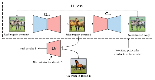 Fig 6. Illustration of the training process for G [5].
Stable Diffusion
Stable Diffusion is in the class of latent diffusion models (LDMs). Similar to diffusion models, LDMs work by repeatedly removing noise from an image, but instead of starting in the pixel space, LDMs start in the latent space.
Why might this be a good idea?
We can reduce the dimensionality with minimal loss of information! This makes training and image generation more efficient and allows for high-resolution image synthesis.
Diffusion Model
Before diving into Stable Diffusion, we start by discussing the fundamental diffusion model. The diffusion model is a parameterized Markov chain trained using variational inference to produce samples matching the data after finite time [1]. The process it divided into two parts: the forward process which adds noise to the original image, and the backward process which gradually denoise the noisy input to get an image.

Fig 7. The diffusion and reverse illustrated as a directed graphical model [1].
In the forward pass, we add noise to the input image following a variance schedule \(\beta_1, ..., \beta_T\). The approximate posterior (diffusion process) is defined as:
\[q(\mathbf{x}_{1:T}|\mathbf{x}_0) := \prod_{t=1}^T q(\mathbf{x}_t|\mathbf{x}_{t-1})\]where
\[q(\mathbf{x}_t|\mathbf{x}_{t-1}) := \mathcal{N}(\mathbf{x}_t; \sqrt{1 - \beta_t}\mathbf{x}_{t-1},\beta_t\mathbf{I})\]The quantity we are maximizing is the variational lower bound (VLB) as seen in VAE models.
The backward denoising process obtains a joint distribution (reverse process), which is defined as a Markov chain with learned Gaussian transitions starting at \(p(\mathbf{x}_T) = \mathcal{N}(\mathbf{x}_T;\mathbf{0},\mathbf{I})\):
\[p_{\theta}(\mathbf{x}_{0:T}) := p(\mathbf{x}_T) \prod_{t=1}^T p_{\theta}(\mathbf{x}_{t-1}|\mathbf{x}_t)\]where
\[p_{\theta}(\mathbf{x}_{t-1}|\mathbf{x}_t) := \mathcal{N}(\mathbf{x}_{t-1}; \mathbf{\mu}_{\theta}(\mathbf{x}_t, t), \Sigma_{\theta}(\mathbf{x}_t, t))\]During the backward process, instead of directly denoising the image, predicting the noise and subtracting it from the image turned out to be a more feasible approach.
While the conventional diffusion model achieves satisfying results by generating high quality images, it directly operates in pixel space, making the training process expensive in terms of computational resources. The sequential evaluation for inference also made the model slow. In order to train on limited computational resources while sacrificing little loss in generated image quality and flexibility, we turn to the Latent Diffusion Model (LDM).
Latent Diffusion Model
Instead of sampling from the pixel space, the Latent Diffusion Model samples from the latent space of a powerful pretrained autoencoder [5]. The autoencoder is universal, and is trained only once in order to apply multiple LDM trainings. The autoencoder is trained by combination of a perceptual loss and a patch-based adversarial objective [5] such that the reconstruction are confined to the image manifold and avoids blurriness if solely relying on pixel space losses.
More formally, the encoder \(\mathcal{E}\) encodes the image \(x \in \mathbb{R}^{H \times W \times 3}\) into \(z = \mathcal{E}(x) \in \mathbb{R}^{h \times w \times c}\), where \(f = H/h = W/w\) is the downsampling factor and is typically an integer power of 2. The decoder \(\mathcal{D}\) decodes input from the latent space back to the dimension of a regular input image: \(\tilde{x} = \mathcal{D}(z) = \mathcal{D}(\mathcal{E}(x))\). After training of the autoencoder is completed, we wrap the whole diffusion process in between the encoder and decoder, so that the diffusion model operates entirely in the latent space.
Training Latent Diffusion Model
A good latent space of lower dimension preserves the most important data of the input image while occupying less space. We define our new objective function for the LDM as follows:
\[L_{LDM} := \mathbb{E}_{\mathcal{E}(x), \epsilon \sim \mathcal{N}(0, 1), t}[||\epsilon - \epsilon_{\theta}(z_t, t)||_2^2]\]where the neural backbone \(\epsilon_{\theta}(z_t, t); t = 1...T\) is an equally weighted sequence of denoising autoencoders. One of the realizations of it is through a time-conditional UNet.
The versatility of LDM allows us to incorporate other conditioning mechanisms, by augmenting the underlying UNet with cross-attention mechanism.
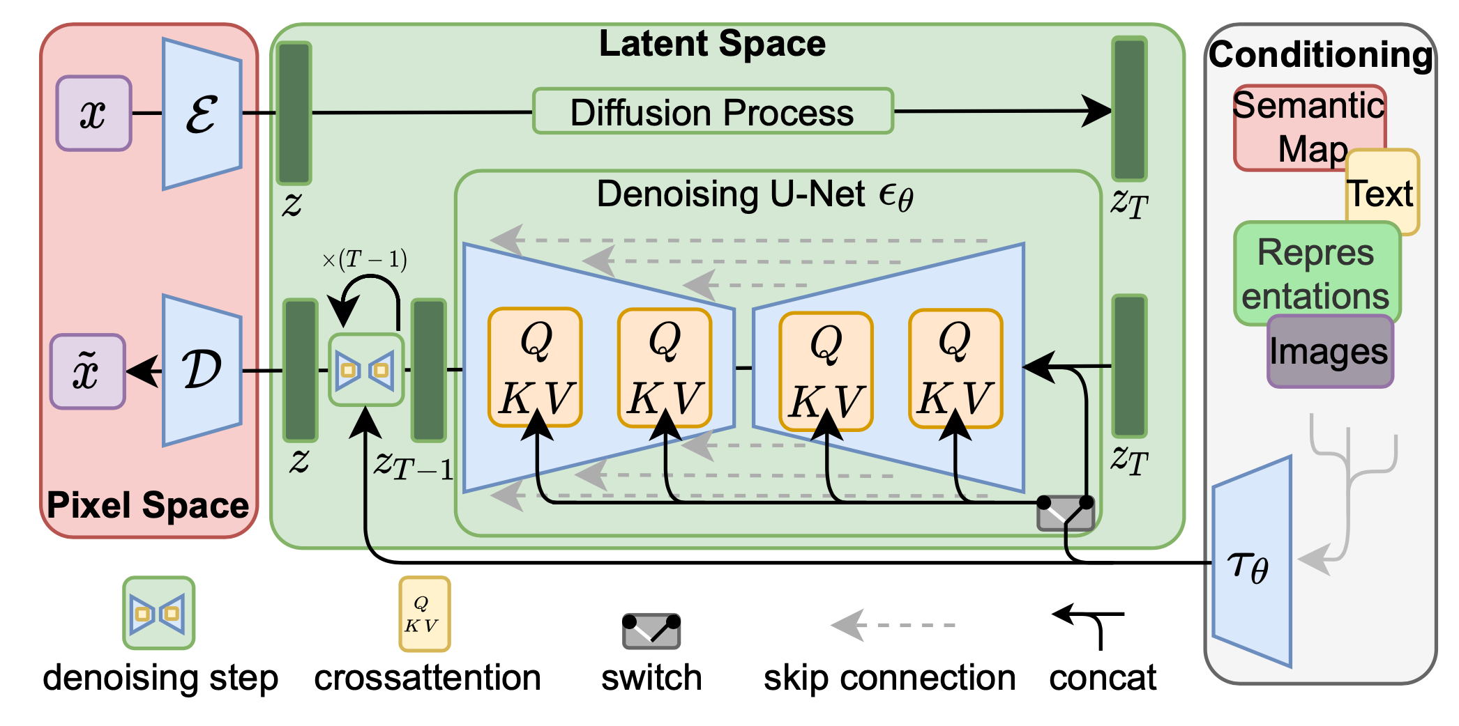
Fig 1. LDM architecture with conditioning [5].
For example, we can add a caption to the LDM to describe the output image, allowing more control over the generated result. In order to account for the multimodal input (such as text captioning), a domain specific encoder \(\tau_{\theta}\) is introduced to project the multimodal input \(y\) to map to the intermediate layers of the UNet via cross-attention layer. The cross-attention layer implements
\[Attention(Q, K, V) = softmax(\frac{QK^T}{\sqrt{d}})\cdot V\]where \(Q\) is obtained using the flattened intermediate representation of the UNet implementing \(\epsilon_{\theta}\), and \(K, V\) obtained via \(\tau_{\theta}(y)\). The new denoising autoencoder now takes an additional input and is expressed as \(\epsilon_{\theta}(z_t, t, \tau_{\theta}(y))\).
Image Captioning with Transformers
To caption an image, we can use a encoder-decoder architecture [2]. To do so, we use a pre-trained Transformer-based vision model as encoder and a pre-trained language model as decoder. The encoder produces an embedding of the image, which can be used by the decoder to generate a caption.
Experimentation: Approaching Realistic Image to Monet-style Painting
We explore two methods to translate realistic images to Monet-style paintings: CycleGAN and our own proposed method using Image Captioning and Stable Diffusion.
Running CycleGAN
We followed the instruction from th github repository of CycleGAN paper and focused on the Monet dataset in particular. We found that the training process was very slow and the results after 100 epochs were not good. We expected this to be due to the difficulty of training GAN models and the complexity of the Monet dataset. Then we downloaded the pretained model fro the authors and tested on test dataset.
# clone the repository
git clone git@github.com:junyanz/pytorch-CycleGAN-and-pix2pix.git
cd pytorch-CycleGAN-and-pix2pix
# download the dataset
bash ./datasets/download_cyclegan_dataset.sh monet2photo
# train the model
python train.py --dataroot ./datasets/monet2photo --name monet_cyclegan --model cycle_gan
# test the model
python train.py --dataroot ./datasets/monet2photo/ --name monet_cyclegan --model cycle_gan --batch_size 8 --epoch_count=1 --n_epochs=50 --n_epochs_decay=50
# download the pretrained model (style to monet)
bash ./scripts/download_cyclegan_model.sh style_monet
# test the pretrained model
python test.py --dataroot datasets/monet2photo/testB --name style_monet_pretrained --model test --no_dropout
Running Stable Diffusion
We used the CompVis sdv1.4 available on Hugging Face for generation. We used the nlpconnect/vit-gpt2-image-captioning available on Hugging Face for image captioning. We first tested on the pretrained model and then fine-tuned on monet dataset.
To translate the image, we first generated the captions of the input using image (photo) captioning model, then we modified the captions to conditioned on Monet style. We then used the stable diffusion model to generate the image (painting) from the modified captions.
# generate
def generate_caption(image, feature_extractor, tokenizer, model):
    pixel_values = feature_extractor(images=image, return_tensors="pt").pixel_values
    pixel_values = pixel_values.to(device)
    output_ids = model.generate(pixel_values)
    caption = tokenizer.decode(output_ids[0], skip_special_tokens=True)
    return caption

def generate_images(folder_path, generate_path):
    pipe = StableDiffusionPipeline.from_pretrained(model_id, torch_dtype=torch.float16).to(device)
    img_caption = VisionEncoderDecoderModel.from_pretrained("nlpconnect/vit-gpt2-image-captioning", torch_dtype=torch.float16).to(device)
    feature_extractor = ViTImageProcessor.from_pretrained("nlpconnect/vit-gpt2-image-captioning")
    tokenizer = AutoTokenizer.from_pretrained("nlpconnect/vit-gpt2-image-captioning")

    for file_name in tqdm(os.listdir(folder_path)):
        if file_name.endswith(('.png', '.jpg', '.jpeg')):
            image_path = os.path.join(folder_path, file_name)
            image = Image.open(image_path).convert('RGB')
            caption = generate_caption(image, feature_extractor, tokenizer, img_caption)
            caption = f'a painting of {caption}by Claude Monet.'
            output = pipe(caption, guidance_scale=5).images
            output[0].save(os.path.join(generate_path, file_name))

# Example usage
device = 'cuda' if torch.cuda.is_available() else 'cpu'
folder_path = './monet2photo/testB/'
# model_id = "CompVis/stable-diffusion-v1-4"
generate_path = './monet2photo/generated_monet_1000/'
model_id = './models/monet-1000/'

generate_images(folder_path, generate_path)
We fine-tuned the t2i stable diffusion model on Monet dataset. We first generated the captions of the Monet paintings then passed the painting, captions pairs to the pretained model for fine-tuning.
# captioning
def generate_caption(image, feature_extractor, tokenizer, model):
    pixel_values = feature_extractor(images=image, return_tensors="pt").pixel_values
    pixel_values = pixel_values.to(device)
    output_ids = model.generate(pixel_values)
    caption = tokenizer.decode(output_ids[0], skip_special_tokens=True)
    return caption

def process_images(folder_path, csv_file_path):
    img_caption = VisionEncoderDecoderModel.from_pretrained("nlpconnect/vit-gpt2-image-captioning").to(device)
    feature_extractor = ViTImageProcessor.from_pretrained("nlpconnect/vit-gpt2-image-captioning")
    tokenizer = AutoTokenizer.from_pretrained("nlpconnect/vit-gpt2-image-captioning")

    data = []

    for file_name in tqdm(os.listdir(folder_path)):
        if file_name.endswith(('.png', '.jpg', '.jpeg')):
            image_path = os.path.join(folder_path, file_name)
            image = Image.open(image_path).convert('RGB')
            caption = generate_caption(image, feature_extractor, tokenizer, img_caption)
            caption = f'a painting of {caption}by Claude Monet.'
            data.append([file_name, caption])

    # Create a DataFrame and save to CSV
    df = pd.DataFrame(data, columns=['file_name', 'text'])
    df.to_csv(csv_file_path, index=False)

# Example usage
device = 'cuda' if torch.cuda.is_available() else 'cpu'
folder_path = './monet2photo/trainA/'
csv_file_path = './monet2photo/trainA/metadata.csv'
process_images(folder_path, csv_file_path)
To fine-tune t2i diffusion, we used the python code from Hugging Face train_text_to_image.py. Here is the script:
export MODEL_NAME="CompVis/stable-diffusion-v1-4"
export TRAIN_DIR="./monet2photo/trainA"
export OUTPUT_DIR="./models/monet-3000"

accelerate launch train_text_to_image.py \
  --pretrained_model_name_or_path=$MODEL_NAME \
  --train_data_dir=$TRAIN_DIR \
  --use_ema \
  --resolution=512 --center_crop --random_flip \
  --train_batch_size=1 \
  --gradient_accumulation_steps=4 \
  --gradient_checkpointing \
  --mixed_precision="fp16" \
  --max_train_steps=3000 \
  --learning_rate=1e-05 \
  --max_grad_norm=1 \
  --lr_scheduler="constant" --lr_warmup_steps=0 \
  --output_dir=${OUTPUT_DIR}
We fine-tuned for 1000 epochs and 3000 epochs. We indeed saw improvement after fine-tuning, and 1000-step and 3000-step tuning did not show significant difference.
FID Score
We calculated the FID score for generated paintings by each model. We use the pytorch-fid as the base code. FID score measures the similarity between two datasets of images.
\[\text{FID}(\mathcal{N}(\mu_1, \Sigma_1), \mathcal{N}(\mu_2, \Sigma_2)) = ||\mu_1 - \mu_2||^2_2 + Tr(\Sigma_1+\Sigma_2-(\Sigma_1\Sigma_2)^{\frac{1}{2}})\]FID score is calculated by finding the statistics of samples activation at the last layer of a image classifier (usually InceptionV3). The lower the FID score, the more similar the two datasets are.
| model | FID score |
|---|---|
| CycleGAN | 61.9179 |
| Stable Diffusion (pretrained) | 85.8571 |
| Stable Diffusion (1000 steps) | 73.5340 |
| Stable Diffusion (3000 steps) | 73.9927 |
Table 1. FID score of generated paintings by each model.
Interestingly, the FID score of the generated paintings by Stable Diffusion was a bit higher than the FID score of the generated paintings by CycleGAN. This may cause by loss of the geometric information when converting the image to text then to image. As expected, after fine-tuning, the FID score of standard diffusion decreased.
Code for calculating FID score:
base_datasets=("/home/zichunl/others/cs188_proj/monet2photo/testA")

target_datasets=("/home/zichunl/others/cs188_proj/monet2photo/generated_pretrained" \
    "/home/zichunl/others/cs188_proj/monet2photo/generated_monet_1000" \
    "/home/zichunl/others/cs188_proj/monet2photo/generated_monet_3000" \
    "/home/zichunl/others/cs188_proj/monet2photo/generated_cyclegan")

base_names=("true_monet")
target_names=("sd_pretrained" "sd_1000" "sd_3000" "cyclegan")

npzs_path="/home/zichunl/fid"

for i in ${!base_datasets[@]}; do
    data=${base_datasets[i]}
    name=${base_names[i]}
    CUDA_VISIBLE_DEVICES=0 python fid_score.py $data /home/zichunl/fid/val_$name \
    --save-stats --num-workers=8 --device=cuda
done

for i in ${!target_datasets[@]}; do
    data=${target_datasets[i]}
    name=${target_names[i]}
    CUDA_VISIBLE_DEVICES=0 python fid_score.py $data /home/zichunl/fid/val_$name \
    --save-stats --num-workers=8 --device=cuda
done

for base_name in ${base_names[@]}; do
    for target_name in ${target_names[@]}; do
        echo "$base_name and $target_name"
        CUDA_VISIBLE_DEVICES=0 python fid_score.py \
        $npzs_path/val_$base_name.npz $npzs_path/val_$target_name.npz \
        --num-workers=8 --device=cuda
    done
done
def get_activations(files, model, batch_size=50, dims=2048, device='cpu',
                    num_workers=1):
    """Calculates the activations of the pool_3 layer for all images.

    Params:
    -- files       : List of image files paths
    -- model       : Instance of inception model
    -- batch_size  : Batch size of images for the model to process at once.
                     Make sure that the number of samples is a multiple of
                     the batch size, otherwise some samples are ignored. This
                     behavior is retained to match the original FID score
                     implementation.
    -- dims        : Dimensionality of features returned by Inception
    -- device      : Device to run calculations
    -- num_workers : Number of parallel dataloader workers

    Returns:
    -- A numpy array of dimension (num images, dims) that contains the
       activations of the given tensor when feeding inception with the
       query tensor.
    """
    model.eval()

    if batch_size > len(files):
        print(('Warning: batch size is bigger than the data size. '
               'Setting batch size to data size'))
        batch_size = len(files)
    mean = [0.485, 0.456, 0.406]
    std = [0.229, 0.224, 0.225]
    transform = TF.Compose([
        TF.Resize((256, 256)),
        TF.ToTensor(),
        TF.Normalize(mean=mean, std=std)
    ])

    dataset = ImagePathDataset(files, transforms=transform)
    dataloader = torch.utils.data.DataLoader(dataset,
                                             batch_size=batch_size,
                                             shuffle=False,
                                             drop_last=False,
                                             num_workers=num_workers)

    pred_arr = np.empty((len(files), dims))

    start_idx = 0

    for batch in tqdm(dataloader):
        batch = batch.to(device)

        with torch.no_grad():
            pred = model(batch)[0]

        # If model output is not scalar, apply global spatial average pooling.
        # This happens if you choose a dimensionality not equal 2048.
        if pred.size(2) != 1 or pred.size(3) != 1:
            pred = adaptive_avg_pool2d(pred, output_size=(1, 1))

        pred = pred.squeeze(3).squeeze(2).cpu().numpy()

        pred_arr[start_idx:start_idx + pred.shape[0]] = pred

        start_idx = start_idx + pred.shape[0]

    return pred_arr

def calculate_frechet_distance(mu1, sigma1, mu2, sigma2, eps=1e-4):
    """Numpy implementation of the Frechet Distance.
    The Frechet distance between two multivariate Gaussians X_1 ~ N(mu_1, C_1)
    and X_2 ~ N(mu_2, C_2) is
            d^2 = ||mu_1 - mu_2||^2 + Tr(C_1 + C_2 - 2*sqrt(C_1*C_2)).

    Stable version by Dougal J. Sutherland.

    Params:
    -- mu1   : Numpy array containing the activations of a layer of the
               inception net (like returned by the function 'get_predictions')
               for generated samples.
    -- mu2   : The sample mean over activations, precalculated on an
               representative data set.
    -- sigma1: The covariance matrix over activations for generated samples.
    -- sigma2: The covariance matrix over activations, precalculated on an
               representative data set.

    Returns:
    --   : The Frechet Distance.
    """

    mu1 = np.atleast_1d(mu1)
    mu2 = np.atleast_1d(mu2)

    sigma1 = np.atleast_2d(sigma1)
    sigma2 = np.atleast_2d(sigma2)

    assert mu1.shape == mu2.shape, \
        'Training and test mean vectors have different lengths'
    assert sigma1.shape == sigma2.shape, \
        'Training and test covariances have different dimensions'

    diff = mu1 - mu2

    # Product might be almost singular
    covmean, _ = linalg.sqrtm(sigma1.dot(sigma2), disp=False)
    if not np.isfinite(covmean).all():
        msg = ('fid calculation produces singular product; '
               'adding %s to diagonal of cov estimates') % eps
        print(msg)
        offset = np.eye(sigma1.shape[0]) * eps
        covmean = linalg.sqrtm((sigma1 + offset).dot(sigma2 + offset))

    # Numerical error might give slight imaginary component
    if np.iscomplexobj(covmean):
        if not np.allclose(np.diagonal(covmean).imag, 0, atol=1e-3):
            m = np.max(np.abs(covmean.imag))
            raise ValueError('Imaginary component {}'.format(m))
        covmean = covmean.real

    tr_covmean = np.trace(covmean)

    return (diff.dot(diff) + np.trace(sigma1)
            + np.trace(sigma2) - 2 * tr_covmean)

def calculate_activation_statistics(files, model, batch_size=50, dims=2048,
                                    device='cpu', num_workers=1):
    """Calculation of the statistics used by the FID.
    Params:
    -- files       : List of image files paths
    -- model       : Instance of inception model
    -- batch_size  : The images numpy array is split into batches with
                     batch size batch_size. A reasonable batch size
                     depends on the hardware.
    -- dims        : Dimensionality of features returned by Inception
    -- device      : Device to run calculations
    -- num_workers : Number of parallel dataloader workers

    Returns:
    -- mu    : The mean over samples of the activations of the pool_3 layer of
               the inception model.
    -- sigma : The covariance matrix of the activations of the pool_3 layer of
               the inception model.
    """
    act = get_activations(files, model, batch_size, dims, device, num_workers)
    mu = np.mean(act, axis=0)
    sigma = np.cov(act, rowvar=False)
    return mu, sigma


def compute_statistics_of_path(path, model, batch_size, dims, device,
                               num_workers=1):
    if path.endswith('.npz'):
        with np.load(path) as f:
            m, s = f['mu'][:], f['sigma'][:]
    else:
        path = pathlib.Path(path)
        files = sorted([file for ext in IMAGE_EXTENSIONS
                        for file in path.glob('**/*.{}'.format(ext))]) # change to '*.{}' for class-wise fid
        m, s = calculate_activation_statistics(files, model, batch_size,
                                               dims, device, num_workers)

    return m, s
Results
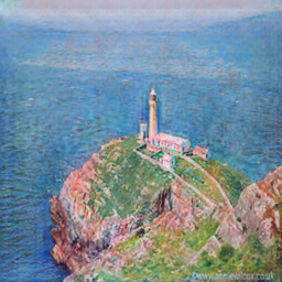
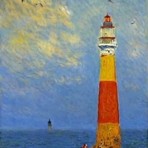
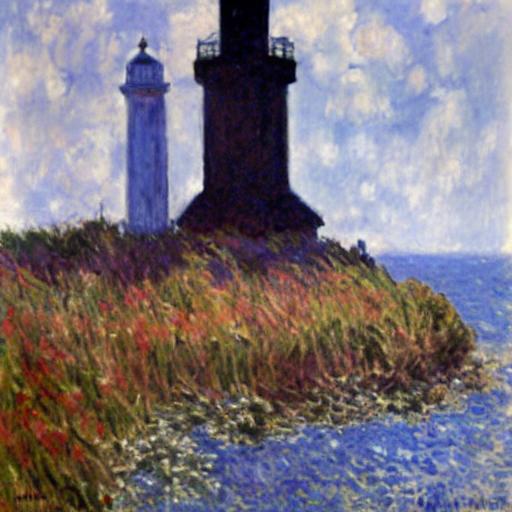
In terms of outputs, the images generated by CycleGAN are geometrically analogus to the input images, so it retains spatial semantics very well. However, the geometric rigidity could limits CycleGAN’s ability to capture more abstract styles that require geometric morphing. Stable Diffusion, on the other hand, generates images that have similar content to the input images but does not retain any spatial semantics. This is due to the fact that Image Captioning does not preserve spatial information. Without the geometric constraints, Stable Diffusion should perform better on translating to styles that require more complex geometric morphing.
| Description | Image 1 | Image 2 |
|---|---|---|
| Input Image (Realistic) | 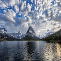 |
 |
| CycleGAN | 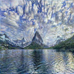 |
 |
| Stable Diffusion (pretrained) | 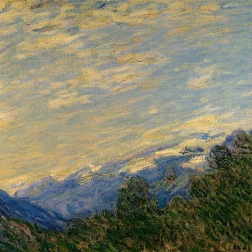 |
 |
| Finetuned SD (1000 epochs) | 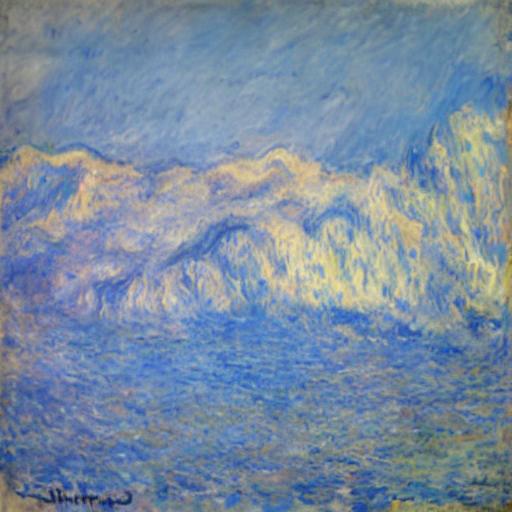 |
 |
| Finetuned SD (3000 epochs) | 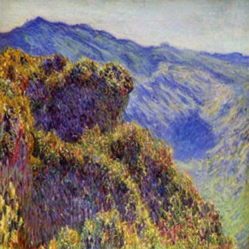 |
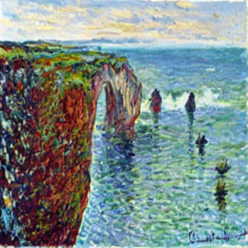 |
Table 2. Comparison of outputs from CycleGAN and Stable Diffusion
Discussion
This section will compare CycleGAN and Stable Diffusion in terms of their architecture, training process, inference speed, flexibility, and also the results of transferring an image to Monet style.
Architecturally, CycleGAN uses a generative adversarial network architecture with two generators and two discriminators. With the unique feature of cycle-consistency, CycleGAN ensures that an image can preserve as much content as possible when converted to another style and back again. Thus, CycleGAN implicitly models the data distribution. On the other hand, Stable Diffusion leverages a Latent Diffusion Model architecture to explicitly compute the distribution. Stable Diffusion combines the concepts from diffusion models and variational autoencoders to ensure efficient encoding and decoding.
For training, CycleGAN is trained on unpaired dataset from two different domains whereas Stable Diffusion is trained on a large dataset of images with their corresponding textual descriptions.
CycleGAN’s inference speed if faster than Stable Diffusion model since the image is generated by passing through the generator once, whereas Stable Diffusion takes many denoising steps to generate an image. However, the training process of CycleGAN can be time-consuming and requires a significant amount of computational power.
In terms of flexibility, CycleGAN is limited, because a CycleGAN model is only trained to transfer between specific domains, which mean we need to retrain the model for each new style. Stable Diffusion, however, offers greater flexibility due to its ability to interpret and apply styles based on textual description.
Although in terms of FID score CycleGAN performed better than Stable Diffusion, many generated images by CycleGAN actually look worse than those by Stable Diffusion. CycleGAN only changes the coloring and edges of the images while keeps most of the geometric information. However, human eyes sometimes are more sensitive to colors. This suggests that Stable Diffusion in terms of this actually performs better than CycleGAN. In the future, we can improve the Stable Diffusion by introducing methods to perserve more spatial information.
Reference
[1] Ho, J., Jain, A. N., & Abbeel, P. “Denoising diffusion probabilistic models.” arXiv (Cornell University). 2020.
[2] Kumar, Ankur. “The Illustrated Image Captioning using transformers.” ankur3107.github.io. 2022.
[3] Redmon, Joseph, et al. “You only look once: Unified, real-time object detection.” Proceedings of the IEEE conference on computer vision and pattern recognition. 2016.
[4] Ronneberger, Olaf, Philipp Fischer, and Thomas Brox. “U-net: Convolutional networks for biomedical image segmentation.” Medical image computing and computer-assisted intervention–MICCAI 2015: 18th international conference, Munich, Germany, October 5-9, 2015, proceedings, part III 18. Springer International Publishing, 2015.
[5] Yuan, Yuan, et al. “Unsupervised image super-resolution using cycle-in-cycle generative adversarial networks.” Proceedings of the IEEE conference on computer vision and pattern recognition workshops. 2018.