Road Agent Behavior and Trajectory Prediction
In this paper, we review various deep learning models that are capable of predicting the future actions of various road actors.
Introduction
Trajectory and behavior prediction is a very prevalent topic in the autonomous vehicle industry since it plays a significant role in developing automated driving systems. One of the biggest challenges is being able to accurately predict and track road actors such as vehicles, pedestrians, and bicycles. Reliable movement predictions become that much more important to an autonomous vehicle, especially on city roads with other traffic. Deep learning models have been successful in mitigating the issue of unreliable trajectory predictions, with CNN-RNN hybrid models being used most commonly. The challenge with many of these models is that they have issues predicting the trajectory of road actors that do not conform to the expected behavior of traffic laws. Actor interaction and behavior classification are both innovations that help mitigate this issue, as we will outline.
In this paper, we will present in depth three deep learning models that tackle the issue of road agent trajectory and behavior prediction. Each model builds off of common CNN architectures and augments them with different techniques. The first model, FastMobileNet, provides a way to efficiently predict the future motion of vulnerable road users (such as pedestrians and bicyclists). The next model is the TraPHic model, which adds weighted actor interactions with LSTMs to a CNN architecture. Finally, the third model is a two-stream graph-LSTM model that incorporates behavior prediction into trajectory prediction by classifying road-agents with three different behaviors based on their movement to better predict their expected trajectories.
For each model, we will outline the motivation behind the design, explain the structure of the architecture, and evaluate the results obtained. Finally, we will conclude on how the different approaches perform and how each presents a promising architectural innovation.
Models
Prediction Motion of Vulnerable Road Users using High-Definition Maps and Efficient ConvNets
Paper: https://arxiv.org/pdf/1906.08469.pdf
Motivation
The motivation behind this paper is the critical need for Self-Driving Vehicles (SDVs) to predict the future motion of Vulnerable Road Users (VRUs). The ability to predict the future motion of a VRU (such as a pedestrian or bicyclist) is extremely important to reduce the risk of injury between a SDV and VRU. VRUs tend to possess a higher risk of injury due to their less predictable movements. This particular implementation uses deep learning to predict VRU movement by rasterizing high-definition maps of the SDVs surroundings into a bird’s-eye view image for input into deep Convolutional Neural Networks (CNNs).
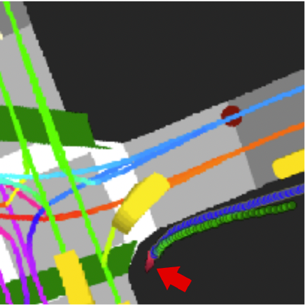
Fig.1 : Example input raster for a pedestrial model.
Structure of the architecture
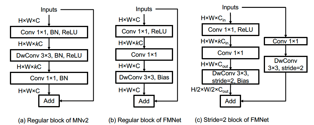
Fig. 2: Building blocks of MobileNet-v2 (MNv2) and the proposed FastMobileNet (FMNet) architecture.
The proposed architecture is a CNN that is designed specifically for fast inference, given the real-time application in SDVs. The architecture is called FastMobileNet (FMNet) and is based on MobileNet-v2 (MNv2), but introduces modifications that increase speed and efficiency, which are critical for running onboard a SDV.
Table 1: Architecture of FastMobileNet
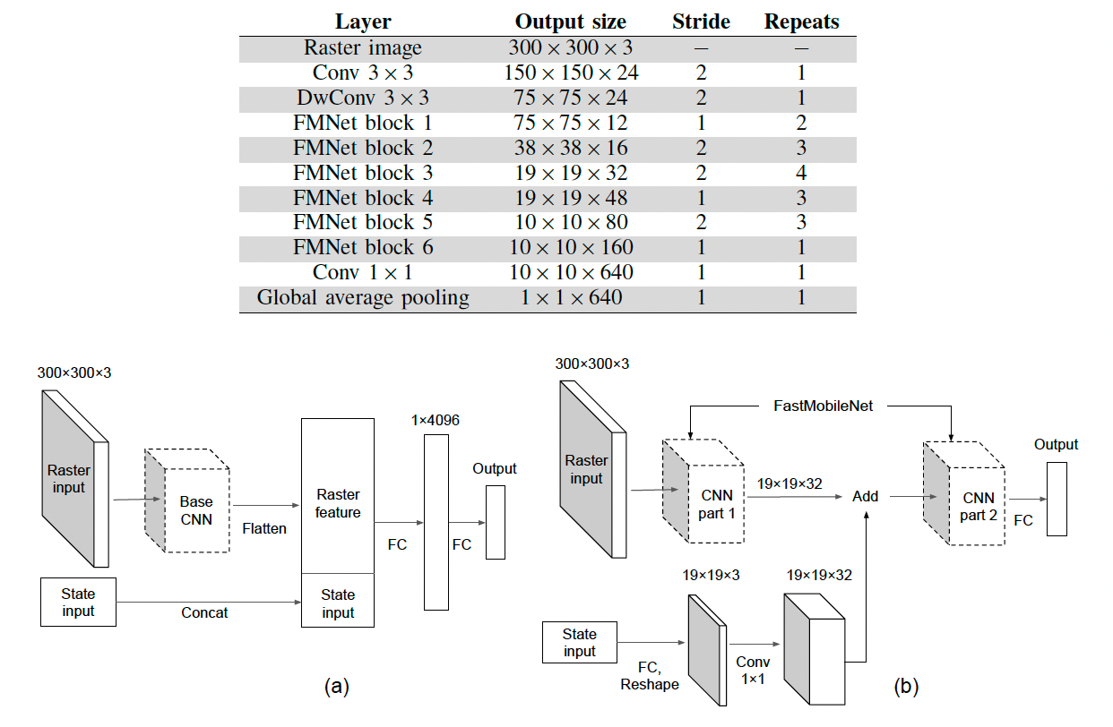
Fig. 3: Feature fusion through (a) concatentation; and (b) spatial fusion.
Original Architecture (MNv2)
The base CNN in MNv2 uses the inverted bottle neck block (illustrated in Fig. 2a). The input feature map is upsampled k times more channels using 1x1 convolutions. It is then passed to a 3x3 convolution. Then, the feature map is reverted back to its original input size and added to the residual connection.
Architecture Improvements
FMNet uses the base CNN from the MNv2 model, while making numerous improvements. One of the first improvements made to the base CNN from MNv2 is refactoring the operations done in the inverted bottleneck block. The operations that were originally done in the upsampling phase have been moved to the bottleneck phase in FMNet. This reduces computational demands and memory access operations by a factor of k. Furthermore, Batch Normalization has been omitted from FMNet due to its minimal impact on model convergence.
To improve model performance, the model can take in both raster input with other state features (such as current velocity, acceleration, heading change rate). Thus, the model takes in the 3D raster image tensor and a 1D auxiliary features tensor. The straightforward approach, done in Fig. 3a, concatenates the flattened CNN output with the 1D auxiliary features tensor. The paper proposes an improvement on this process, by fusing together the CNN output with the auxiliary features. The 1D auxiliary feature tensor is converted to a 3D tensor by a fully-connected layer, then fed into a convolutional layer. The output of this layer is then element-wise added to the output of the base CNN. This improvement over the straightforward concatenation approach allows us to not add any additional fully connected layers.
Rasterization
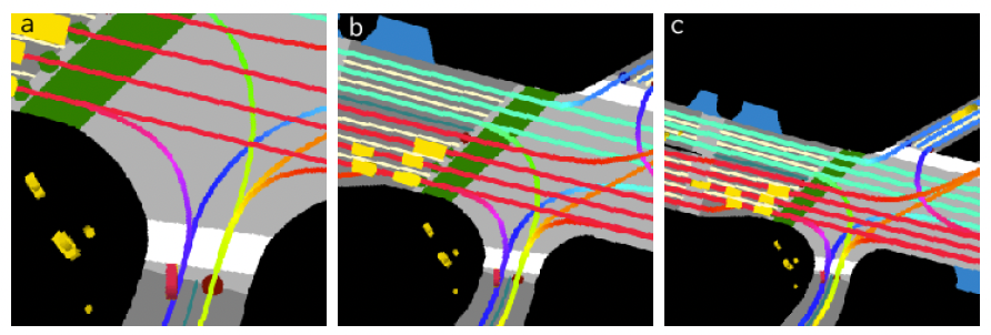
Fig. 4: Raster images for bicyclist actor (colored red) using resolutions of 0.1m, 0.2m, and 0.3m, respectively.
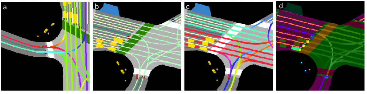
Fig. 5: Different rasterization settings with 0.2m resolution for a cyclist examples: (a) no raster rotation, (b) no lane heading encoding, (c) no traffic light encoding, (d) learned colors
Given that one of the inputs to this model is a rasterized image, it is important to understand rasterization and the impact of different rasterization techniques. Before rasterizing, we need to obtain a vector layer, which is a collection of polygons and lines that belong to a specific type. For example, we may have a vector layer of roads, crosswalks, and other map features. The vector layer is then rasterized to an RGB space, where each vector layer is assigned a unique color. Then iteratively, the vector layers are rasterized on top of one another, starting with the largest elements (such as road boundaries). The study discusses different rasterization techniques, using a RGB raster dimension of 300x300 pixels (n = 300). With regards to resolution, the larger the resolution, the larger the context around the actor (SDV) is captured.
One of the first aspects to consider when rasterizing is the raster pixel resolution. In general, the larger the resolution, the more context that is contained within the rasterized image. Moreover, there is the raster frame rotation, which determines the preset orientation of the actor in the image. For example, we could have a fixed north-up orientation, or an orientation where the actor’s front heading is pointed up. Thirdly, the direction of each lane segment can be optionally encoded into the rasterization using different hue values. For example, we can see in Fig. 4b how lane color indicates heading, where in Fig. 5b it does not. Traffic lights are another aspect which could be encoded into the image. In Fig. 5c, raster images do not encode traffic lights, where in Fig. 4b it does. Lastly, during the generation of raster images, the colors can either be manually chosen or automatically chosen through a learned network.
Results
Table 2: Comparison of various CNN architectures (all models except the last one use the concatenation feature fusion)
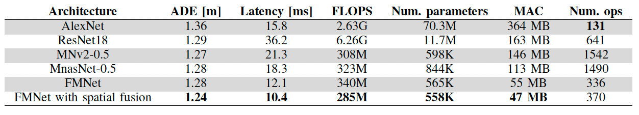
Table 3: Comparison of prediction displacement errors (in meters) for different experimental settings.
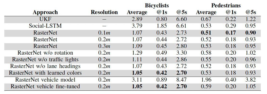
The FMNet demonstrated comparable or better accuracy in predicting VRU motion when compared with other CNN architectures, like MNv2. But, FMNet was notably faster in inference times, accomplishing its mission of being suitable for real-time applications. After analyzing the performance of different resolutions, it was found that 0.1m resulted in lower error for pedestrians, while 0.3m gave the worst performance. Furthermore, 0.3m resulted in slightly higher error for bicyclists, while 0.1m did not show much of an impact. With regards to rotating the rasters, it was found that not rotating rasters (where the actor heading was not pointing up), resulted in a drop of accuracy. Lastly, it was observed that without traffic light rasterization, error increased. After extensive evaluation, the system was successfully deployed on SDVs.
TraPHic: Trajectory Prediction in Dense and Heterogeneous Traffic Using Weighted Interactions
Paper: https://arxiv.org/pdf/1812.04767.pdf
Motivation
The motivation behind the TraPHic model is to better utilize road actor interactions to predict their behavior and trajectory. Often, this prediction task is done using LSTMs that consider each sequence independently, which is not ideal when trying to predict movements when many road actors are present. This challenge is especially difficult in cities with dense traffic or in areas where many different kinds of road actors are present, such as vehicles, pedestrians, bicycles, and so on. To solve this problem, TraPHic uses multiple layers that combine LSTM outputs into maps then pass them through multiple convolution layers to form a more comprehensive model, which allows more accurate trajectory prediction based on the weight of each interaction with respect to the ego vehicle.
Architecture
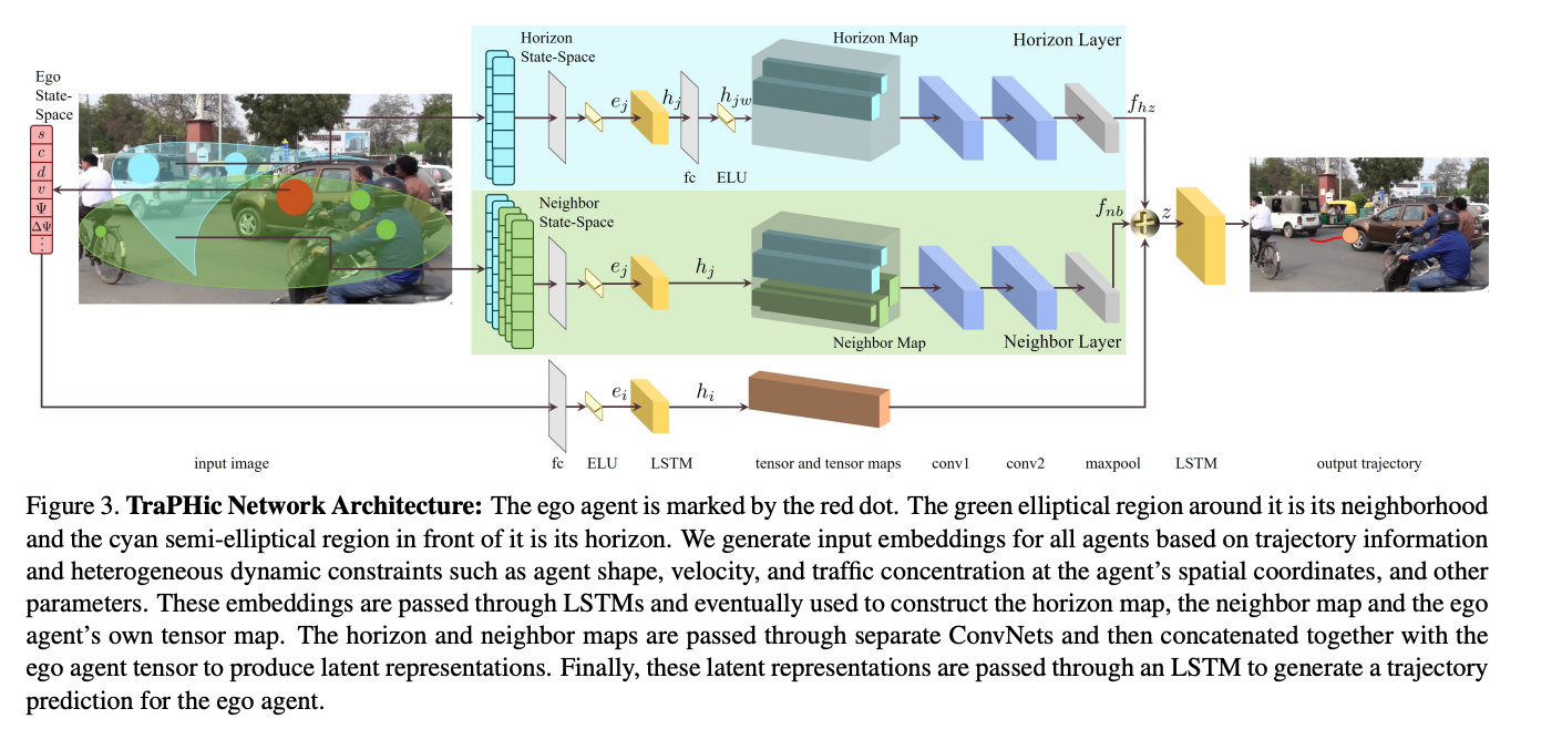
Fig. 6: TraPHic Network Architecture
The traphic model architecture is a CNN-LSTM hybrid that takes advantage of the sequential processing of RNNs while also utilizing CNNs ability to understand feature interactions. Additionally, the use of long short term memory blocks allow the model to more accurately predict trajectory by allowing it to take into account a longer time span than a normal RNN block would.
Weighted Interactions
A defining design distinction of the TraPHic architecture is how it learns weights for road agent interactions and bases them both on implicit constraints of driving behaviors and road actor dynamics. Information such as aggressiveness of conduct, possible turn radius, type of road actor, and distance between actors are embedded into the input. This pre-processing allows the model to learn the relative importance of relationships between road actors based on their intrinsic factors. This improves the model’s ability to understand how heterogeneous interactions will impact the ego vehicle, especially when compared to the classical approach of treating all road actor interactions the same regardless of these factors. Additionally, by weighting the interactions relative to these constraints as well as relative to the distance from the ego vehicle’s path, the model effectively reduces the impact of irrelevant features on the final prediction.
State Space
The key innovation used in the TraPHic architecture is the distinction made between different feature layers and how the outputs of these layers are utilized with different weights in the final prediction. In particular, the architecture divides the input processing into three parts. The first is the neighbor state space, which learns road actor interaction weights within an elliptical horizon around the ego vehicle. This allows for the weights to depend on the relative relationships between the road actors as well as their respective constraints within a large feature space around the ego vehicle and is determined through a nearest neighbor algorithm. The second part is the horizon state space which focuses on learning based on the interactions of the ego vehicle and its neighbors in its path, producing a prioritization of road actor interactions with respect to how directly they impact the ego vehicle. Finally, the last part deals only with the ego vehicle and it models the ego vehicle’s trajectory and behavior. Each of these parts are processed independently through a CNN-LSTM hybrid network then concatenated and passed through a final LSTM block, leading to a prioritization of weights in the horizon feature map and a de-prioritization of weights in the neighbor feature map.
Structural Design
Each feature space layer begins with a fully connected layer, followed by an exponential linear unit (ELU) activation layer. This output is then passed through a single layer LSTM block with 64 hidden layers, producing the hidden state vectors for each layer.
The horizon layer passes the output from this initial set of layers into another fully connected layer followed by an ELU layer, while the neighbor layer and the ego layer pass the output directly in the pooling step. The hidden vectors are pooled into feature maps, the horizon map \(H_i\), the neighbor map \(N_i\), and the ego map \(h_i\) respectively. Both the horizon and neighbor layer then pass their maps through two convolution layers followed by a max pooling operation to form the feature vectors \(f_{hz}\) and \(f_{nb}\). Finally, the three feature vectors \(h_i\), \(f_{hz}\), and \(f_{nb}\) are concatenated into z, which is passed through a final LSTM layer to decode the feature encodings into a trajectory prediction sequence.
Results
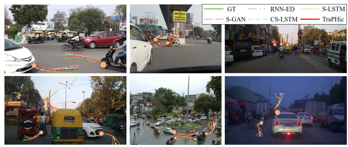
Fig. 7: Trajectory prediction results.
The model was compared to a few common approaches, namely a sequence to sequence RNN encoder used for vehicle trajectory prediction (RNN-ED) and a convolutional social LSTM used for sparse trajectory prediction.
Using the NGSIM dataset, which represents sparse homogenous traffic conditions, the TraPHic model does not perform better than commonly used trajectory prediction models. However, it performs significantly better on a dense heterogeneous traffic dataset compared to other models, with an average displacement error of 0.78 compared to the next lowest error of 1.15 from the CS-LSTM.
Comparing the performance of common models to the TraPHic model unveils an important discrepancy in the design of current trajectory prediction models, which tend to focus primarily on interactions between small amounts of similar road actors and cannot be accurately applied to scenes with many varied actors. Thus, the innovations presented with weighted interactions using implicit behavior and constraint factors is very pertinent to the future development of trajectory prediction models, especially in terms of developing autonomous vehicles.
Forecasting Trajectory and Behavior of Road-Agents Using Spectral Clustering in Graph-LSTMs
Paper: https://arxiv.org/pdf/1912.01118.pdf
Motivation
Trajectory prediction is an active area of research, as it is crucial for safe navigation in autonomous driving. However, current autonomous vehicles are unable to perform efficient navigation in dense and heterogeneous traffic because of the lack of progress in research towards behavior prediction. Furthermore, traffic forecasting possesses a major challenge in ensuring accurate long-term predictions (3-5 seconds) since correlation of the data between the time-steps grows weaker as the margin of time increases. To solve these problems, the paper seeks to contribute a two-stream graph-LSTM network for traffic forecasting in urban traffic, where the first stream does not account for neighboring vehicles and the second stream serves as the behavior prediction and regularization of the first stream. Additionally, the paper proposes spectral cluster regularization for the reduction of long-term prediction errors, a theoretical upper bound of the regularized forecasting algorithm, and a rule-based behavior prediction algorithm to classify a road-agent’s traffic behavior as aggressive, conservative, or neutral.
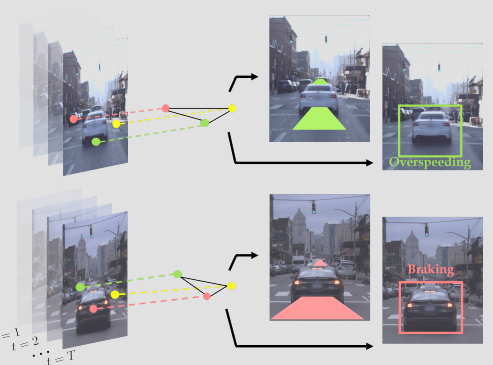
Fig. 8: Represent the spatial coordinates of road-agents as vertices of a dynamic geometric graph (DGG) to improve long-term prediction and predict the behavior of them
Structure
First, the paper defines the problem statement by presenting a definition of a vehicle trajectory. “The trajectory for the i-th road-agent is defined as a sequence \(Ψ_i{}(a,b)\in {\mathbb{R}^{2}}\) where \(Ψ_i(a,b)={[x_t,y_t]^{\top}|t\in [a,b]}.[x,y]\in \mathbb{R}^{2}\) denotes the spatial coordinates of the road-agent in meters according to the world coordinate frame and t denotes the time instance.” Then, it proceeds to define what we intend to predict with the trajectory and the prediction, which is “given the trajectory \(Ψ_i(0,τ)\), predict \(Ψ_i(τ^{+},T)\) for each road-agent \(v_i, i\in[0,N]\)” and “given the same trajectory, predict a label from {Overspeeding, Neutral, Underspeeding} for each road-agent \(v_i, i\in[0,N]\)”. With these definitions in play, the main intentions of the architecture are defined in predicting the trajectory and behavior of each road-agent, which will assist the autonomous vehicle’s ability to determine the long-term trajectory of all the neighboring road-agents.
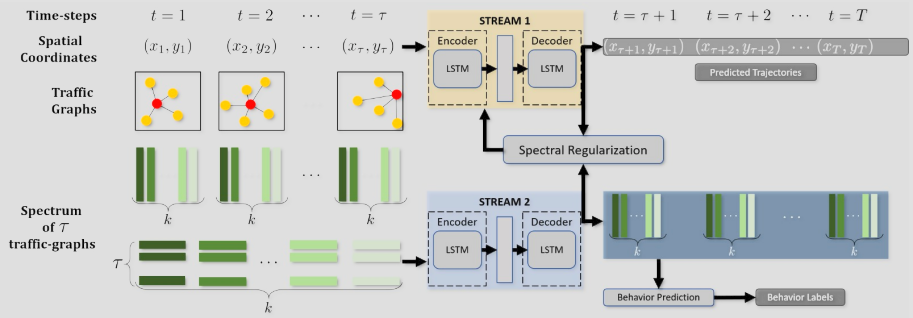
Fig. 9: The trajectory and behavior prediction of the i-th road-agent. Input consists of the spatial coordinates and over the past τ seconds and eigenvectors of the DGGs corresponding to the first τ DGGs. Spectral clustering on the eigenvectors from the second stream to regularize the original loss function and perform back-propagation on the new loss function for improved long-term prediction
Next, the overall flow of the approach must be set, following the figure 9 above: input consists of the spatial coordinates over the past τ seconds and the eigenvectors of the DGGs corresponding to the first τ DGGs. Then, the trajectory prediction problem must be solved through the first stream, using an LSTM-based sequence model. The behavior prediction problem can be solved by accepting the eigenvectors of the input DGGs and predicting the eigenvectors corresponding to those DGGs for the next τ seconds, which form the input to the behavior prediction algorithm. Finally, stream 2 can regularize stream 1 using a new regularization algorithm, which can be used to derive the upper bound on the prediction error of the regularized forecasting algorithm.
Behavior Prediction Algorithm
The defined algorithm for behavior prediction is as below:
- Form the set of predicted spectrums from stream 2 and compute the eigenvalue matrix
- For each set of predicted spectrums, compute the Laplacian matrix
- \(θ_i\) is set to the i-th element of the diagonal matrix operator on the Laplacian matrix
- \(θ_i'\) is equal to the change in \(θ_i\) over time With some preset threshold parameters, some rules can be set to determine the behavior of a road-agent as either overspeeding, neutral, or underspeeding based on the final \(θ_i'\) value.
Spectral Clustering Regularization
The original loss function of stream 1 is given by \(F_i=-\sum_{t=1}^{T}logPr(x_{t+1}|\mu_t,\sigma_t,\rho_t)\). With the goal of optimizing the parameters \(\mu_t^{*},\sigma_t^{*}\) to minimize the above loss equation , there is an issue of predicted trajectory diverging gradually from the ground truth, causing error-margins to increase as time passes. Therefore, a new regularization algorithm is introduced as below to tackle this issue:
- Stream 2 computes a spectrum sequence
- For each spectrum, perform clustering on the eigenvector corresponding to the second smallest eigenvalue
- Compute cluster centers from the clusters obtained from step 2
- Identify the cluster to which each road-agent belongs and retrieve the cluster center and deviation
Upper Bound for Prediction Error
Finally, an upper bound on the prediction error of the first stream must exist. LSTMs make accurate sequence predictions if elements of the sequence are correlated across time, but eigenvectors may not be correlated across time in a general sequence. The goal of this step is to show there exists a correlation between the Laplacian matrices across time-steps with a lower-bound to prove accurate sequence modeling.
Results
By using both sparse and dense datasets (NGSIM, Lyft Level 5, Argoverse Motion Forecasting, and Apolloscape Trajectory), we can witness the benefits of combining behavior prediction into trajectory prediction. The results were determined using the Average Displacement Error(ADE) and the Final Displacement Error (FDE) and compared our model to other methods including CS-LSTM, TraPHic, Social-GAN, and GRIP. All methods that are trajectory prediction models that do not involve any behavior prediction.
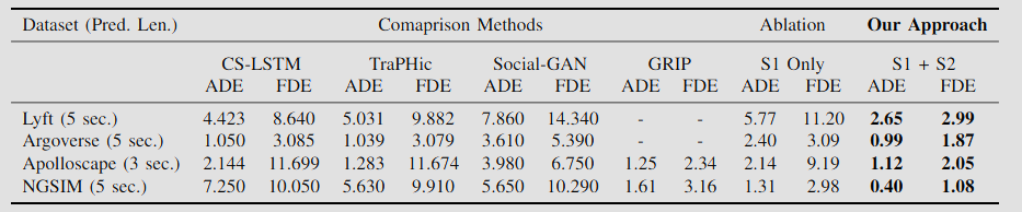
Fig. 10: The main results are as above, showing the ADE and FDE of all the different compared models, with the two-stream graph on the very right
Without a doubt, the results show that there is the least average displacement and final displacement error on the behavior prediction stream model, especially with the behavior prediction included. The final result brags an average and final displacement error clearly below 3 for all the datasets, which is only rivaled by the GRIP method. Finally, when discussing the behavior prediction accuracy, the paper observed a weighted accuracy of 92.96% on the Lyft dataset, 84.11% on the Argoverse dataset, and 96.72% on the Apolloscape dataset. With the high accuracy of the behavior algorithm introduced to the first stream that only performs trajectory prediction, there is great benefit to the final trajectory prediction values as demonstrated by the results above.
Result Comparison
This section will go over a detailed comparison of the three models covered above: FastMobileNet (FMNet), TraPHic, and a two-stream Graph-LSTM model. The comparison will cover the different approaches and applications of each model.
The FastMobileNet (FMNet) model, an adaptation of MobileNet-v2, is specifically tailored for the high-speed inference required by Self-Driving Vehicles (SDVs). The FMNet model focuses on efficiently predicting the movements of Vulnerable Road Users (VRUs). FMNet introduces significant modifications to the original MobileNet-v2 architecture.. This is achieved through the feature fusion approach that allows the model to process raster input alongside other state features, such as velocity and acceleration, without necessitating additional fully-connected layers. Additionally, FMNet employs different rasterization techniques, enabling the model to adaptively capture the contextual environment surrounding the SDV through varied resolutions and rasterization settings.
The TraPHic model introduces a novel approach to handling the intricate dynamics of dense and heterogeneous traffic environments. Its key advantage is the incorporation of weighted interactions among road actors, significantly enhancing the accuracy of trajectory predictions. This model employs a hybrid CNN-LSTM architecture, which leverages the sequential processing strength of RNNs and the feature interaction capabilities of CNNs, facilitating a nuanced understanding of road actor movements.
The Two-stream Graph-LSTM model works by integrating behavior prediction into the trajectory forecasting process. The model operates by using two streams: one focused on trajectory prediction without considering neighboring vehicles, and the second stream serving both as a behavior predictor and a regularizer for the first. This dual-stream approach gives the model the ability to refine its trajectory predictions based on road agement behavior. Road agent behavior is classified as either: aggressive, conservative, or neutral. The model takes advantage of spectral cluster regularization that notably reduces long-term prediction errors.
Each of the discussed deep learning models presents a set of advantages tailored to specific challenges in the realm of autonomous driving systems. FastMobileNet shines with its focus on speed and efficiency, making it ideal for real-time applications requiring the prediction of VRU motion. The TraPHic model stands out for its innovative treatment of weighted interactions, offering robust performance in complex, dense traffic environments. Meanwhile, the two-stream Graph-LSTM model provides a holistic approach by incorporating behavior prediction, promising enhanced accuracy in long-term forecasting.
Conclusion
The study of road agent behavior and trajectory prediction through three distinct deep learning models demonstrates the diversity of solutions to this problem. Each model: the FastMobileNet (FMNet) for predicting the motion of Vulnerable Road Users (VRUs) using high-definition maps and ConvNets, the TraPHic model for trajectory prediction in dense and heterogeneous traffic, and the two-stream graph-LSTM model for forecasting the trajectory and behavior of road-agents, demonstrates unique strengths and architectural innovations tailored to address specific challenges in trajectory and behavior prediction.