An Analytical Dive into What FID is Measuring
Frechet Inception Distance (FID) is a metric that measures the similarity between two sets of images as a distance. It is the gold standard today for quantitative measurement of the performance of generative models such as Generative Adversarial Networks (GANs). Qualitative inspection is often overlooked in GAN research, especially on bad samples generated. In this work, manually inspect approximately 40,000 GAN-generated images and pick 159 good-bad sample pairs, each of which we confirm to be close variants of the same image. We present an analysis of human perceived image quality with respect to variations in FID scores using simple discard and replace schemes. We then analyze FID’s focus on images using Grad-Cam-based visualizations of the selected pairs. Our results urge against relying solely on FID for the evaluation of generators and highlight the need for additional assessment during evaluation.
- 1 Introduction
- 2 Background Knowledge
- 3 Catastrophic Failures
- 4 FID’s Attention
- 5 Conclusion and Future Work
- References
1 Introduction
Generative Adversarial Networks (GANs) [1] have attracted a lot of research interest, and many GAN-based image synthesis models were proposed [2]–[6] for their capability in modeling and generating photo-realistic images. Due to the formulation of GANs, which lacks an objective function, measuring and comparing the performances of learned generators becomes a challenging problem. Quantitatively, the two most common one-dimensional evaluation metrics for GANs are Inception Score (IS) [7], which is deficient in modeling intra-class diversity, and the improved Frechet Inception Distance (FID) [8]. More recently, [9] proposed to use Precision and Recall (P&R) to disentangle the measurement into two metrics: (1) precision, which measures the quality, and (2) recall, which quantifies coverage. Most noteworthily, all of these metrics are based on Convolutional Neural Networks (CNNs) trained on the ImageNet dataset [9], [10], which have shown to concentrate on local textures rather than general shapes [11]. However, these metrics, especially FID, are still used extensively due to their summarizing power and empirical success [12]. On the other hand, qualitative analyses of GAN-generated images are usually overlooked, as researchers tend to sample and present only the good results. To our knowledge, the only two works incorporating qualitative manual inspection are [13], [14]. In this work, we aim to present an analysis of human perceived image quality with respect to variation in FID scores.
This paper is organized as follows. Section 2 presents relevant background knowledge, including the network and dataset used, the FID metric, and the name of spaces used throughout this paper. In Section 3, we sample and present generated good and bad sample pairs and experiment on how these cherry-picked samples affect the FID metric. To be more specific, we compare the three sets of data: (1) the original generated, (2) bad samples discarded, and (3) bad samples replaced with improved but similar ones. We show empirically that in these modifications, even when the human perceived image quality is improved significantly, it is likely that the FID would worsen. In Section 4, we try to understand the behavior of FID by incorporating Grad-Cam [15] based visualization to see where FID is looking during calculation [16]. We present our findings on FID’s focus preference by comparing the FID’s attention on good and bad sample pairs picked from the previous section. Finally, in Section 5, we highlight possible future works.
2 Background Knowledge
2.1 Network and Dataset
The original StyleGAN [3] was introduced as a continuation of the Progressive GAN (PG-GAN) [2]. After that, a family of StyleGANs was proposed [4]–[6]. Figure 1 illustrates the key differences between a style-based generator and a traditional one, such as PG-GAN. Style-based GANs no longer take latent codes directly. Instead, it maps the latent codes into an extended feature space before directing them into the synthesis network. Moreover, this design has an additional source of randomness, called the noise layer. We shall explain the difference between latent and extended latent spaces further in Section 2.3.
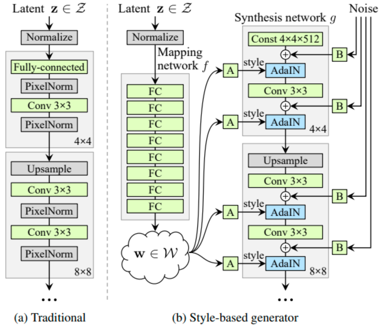
[Figure 1. (a) Traditional generator architecture, seen in, for example, PG-GAN [2]. (b) Illustration of \(z\) space and \(w\) spaces inside the style-based generator architecture. Image from the original StyleGAN [3].]
Many high quality human face image datasets exist [3], [4], [17], [18]. In this paper, our experiments focus on the two datasets, MetFaces [4] and FFHQ [3]. The MetFaces [4] dataset consists of only 1,336 images cropped from images of art collections in the Metropolitan Museum of Art in New York. Images in this dataset are extremely high quality, mostly from famous paintings with a few exceptions, such as sculptures and the Egyptian Pharaoh. The 70,000 images in the FFHQ [3] dataset are collected from the Flickr website and contain considerable variations in age, ethnicity, background, accessories worn, et cetera. Images are also high-quality, thanks to their dlib-based preprocessing scheme and human verification via Amazon Mechanical Turk. See Figure 2 for examples from the two datasets.
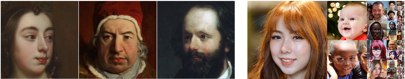
[Figure 2. (left) Samples of MetFaces Dataset [4]. (right) Samples of the FFHQ dataset [3].]
2.2 Frechet Inception Distance
The FID [8] is a metric defined between two data sets that summarize their similarity as a distance metric. Computation of FID first embeds the two sets of images into a feature space from a specific layer of the Inception network [19], [20]. The two sets of embeddings are then viewed as continuous multivariate Gaussian distributions, each with a computed sample mean vector and a covariance matrix. In evaluating GANs, the two sets of data passed into FID computation will be real and generated data, called \(r\) and \(g\), respectively. Let us denote the sample mean vectors as \(\mu_r, \mu_g\) for real and synthetic images, respectively, and similarly for the covariance matrices \(\Sigma_r, \Sigma_g\). The FID is then defined as the Frechet distance between these Gaussian distributions, computed as
\[\mathrm{FID} (r, g) = ||\mu_r - \mu_g||^2_2 + \mathrm{Tr} (\Sigma_r + \Sigma_g - 2(\Sigma_r \Sigma_g) ^{1/2} )\]It is worth noting that FID is bounded below by zero, and the smaller the FID value, the closer the two sets of images.
2.3 Latent and Extended Latent Spaces
This paper widely uses two common style-based GAN [3]–[6] concepts, called \(w\) space and \(z\) space. The \(z\) space stands for the original noise vector as the raw input to the GAN network, which usually follows a high dimensional Gaussian Distribution and may not contain explicit semantic information. On the other hand, the extended latent space, called \(w\) space, is where most linear operations happen. \(w\) space features are the output from the mapping network with the input in \(z\) space. The \(w\) space features are further passed into the synthesis network, consisting of convolution operations. Figure 1(b) illustrates the relationship between these two spaces and their connection to the later synthesis network.
3 Catastrophic Failures
In this paper, we experiment with three GAN models, each (pre-)trained and evaluated on two different human face datasets, for six experiments. All three GAN models that we picked here are from the StyleGAN family, namely StyleGAN2-ADA [4], StyleGAN3-T, and StyleGAN3-R [6]; and the two datasets are FFHQ [21] and MetFaces [4]. We highlight that the linear nature of the extended latent spaces of these models is suitable for our filtering scheme detailed in Section 3.2, which is a fundamental reason we chose to experiment with StyleGAN2-ADA [4], StyleGAN3-T, and StyleGAN3-R [6]. Moreover, using these recently proposed networks allows us to work with generators with relatively small amounts of bad samples, which is crucial to the manual inspection method we introduce. On the other hand, facial images allow a much more straightforward definition of “good” and “bad” samples for humans and reduce the subjectivity involved when compared to, for example, artistic images. We shall illustrate this further in a later section.
3.1 Picking the Pairs
For each GAN model and dataset combination, we generate and pick our good-bad sample pairs as follows.
- We sample seed in the \(z\) space of the generator and generate a total of 1,000 samples.
- Out of the 1,000 samples, we record seeds that contain significant visual defects. Our experiments found approximately 20 - 30 examples for each model-dataset configuration falling into this category.
- For each bad seed we recorded in step 2, we probed around in a small area and generated 200 samples each. Via manual inspection, we identify good-bad pairs inside these 200 images. A bad seed here corresponds to an image with a severe visual defect as usual. In contrast, a good seed corresponds to an image with significant visual improvement and is maximally similar to the bad-seed generated image.
| Model | Dataset | PKL | Num Seed Pairs |
|---|---|---|---|
| StyleGAN3-T | FFHQ | stylegan3-t-ffhq-1024x1024.pkl | 26 |
| StyleGAN3-T | MET | stylegan3-t-metfaces-1024x1024.pkl | 30 |
| StyleGAN3-R | FFHQ | stylegan3-r-ffhq-1024x1024.pkl | 26 |
| StyleGAN3-R | MET | stylegan3-r-metfaces-1024x1024.pkl | 30 |
| StyleGAN2-ADA | FFHQ | ffhq.pkl | 28 |
| StyleGAN2-ADA | MET | metfaces.pkl | 19 |
[Table 1. Summary of picked pairs for each model - dataset pair.]

[Figure 3. Example good bad sample pairs from all six dataset and model pairs. Rows (a) and (c) are bad samples containing apparent visual defects. Rows (b) and (d) are improved samples selected in a small neighborhood close, in \(z\) space, to (a) and (c) respectively.]
Using the procedure, we generated and inspected approximately 40,000 samples, yielding 159 good-bad seed pairs. Table 1 summarizes the number of final picked pairs for each model and dataset combination, and Figure 3 presents a subset of good and bad pairs picked using the procedure outlined above.
3.2 What Can We Do with These Pairs?
With these defined pairs, the easiest and most intuitive way to improve the generator is to discard samples from neighborhoods closer to the picked bad samples than good ones or replace the bad ones with some corresponding good ones.
To evaluate the performance of these simple ideas, we define metrics \(d_i\) for every generated image corresponding to the \(w\) space feature as the distance differences between the good examples and bad examples. In mathematical terms,
\[d_i = ||w_i - \sum_{w \in W_{bad}} \frac{w}{ | W_{bad} | } || - ||w_i - \sum_{w \in W_{good}} \frac{w}{ | W_{good} | } ||\]The larger \(d_i\) is, the relatively closer sample \(i\) is to bad examples. Here, we auto-select all the bad examples with the smallest 1.5% distance \(d_i\). For replacing a bad example selected with a better variant, we modify \(w_i\) to \(w_i’\) as follows:
\[w_i’ = w_i + \sum_{w \in W_{good}} \frac{w}{|W_{good}|} - \sum_{w \in W_{bad}} \frac{w}{|W_{bad}|}\]We run the replacement scheme on the StyleGAN2-ADA generator trained with the MetFaces dataset to assess the quality of the replacement images generated this way. Then, we invite a human expert to perform blind judgment on whether the generated improved image is (1) of better quality than the original and (2) is similar enough to the original image to be called a variant. Out of the 31 sample pairs generated, 30 are rated affirmative that they are variants of the same image. Moreover, 16 out of 31 sample pairs are tagged as a significant improvement by replacement.
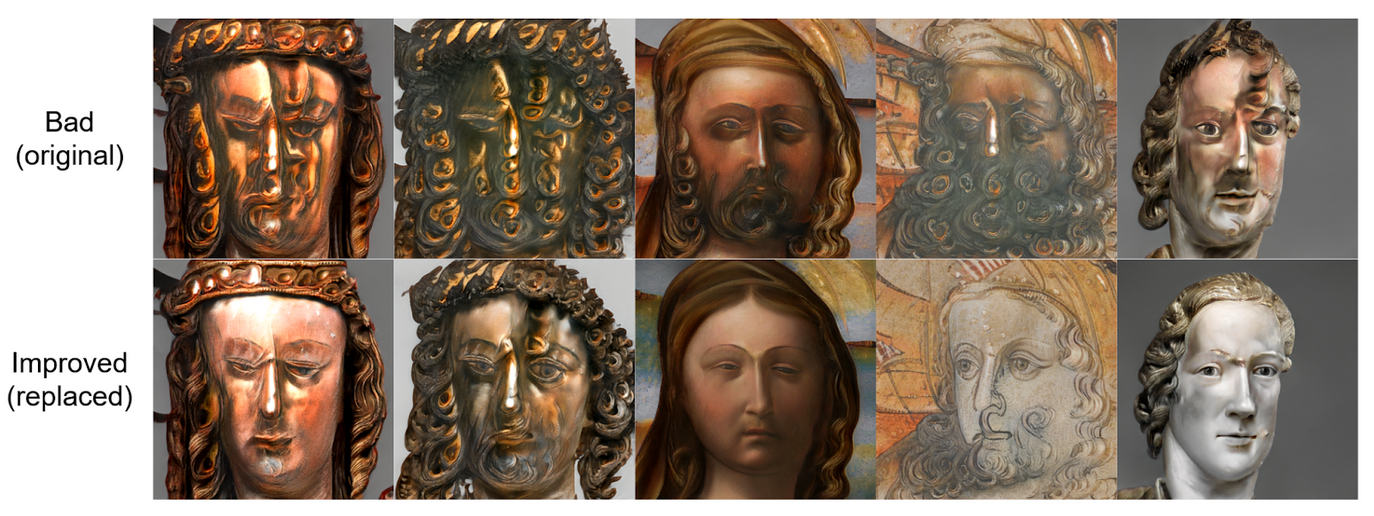
[Figure 4. Example pairs of auto picked bad samples as well as corresponding improved images generated using the scheme described above. The Images shown here are from StyleGAN2-ADA with MetFaces. Top row consists of bad images computed as those with the smallest distance two predefined bad seeds in \(w\) space. Bottom row illustrates improved samples using the scheme detailed above.]
We define two evaluation metrics for the 50k generated images as FID_Replace and FID_Delete, to be compared to the original FID. FID_Replace tries to replace all the bad examples with improved examples, and FID_Delete tries to delete all the bad examples selected. Besides, to show that the better variants generated are indeed of better quality, we further measure FID_Sub_Bad and FID_Sub_Good. FID_Sub_Bad measures the FID distance between the original training dataset and the filtered 1.5% bad samples. In contrast, FID_Sub_Good measures the FID distance between the original training dataset and the generated better variants of the bad samples.
| Dataset | Model | FID | FID_Replace | FID_Delete | FID_Sub_Good | FID_Sub_Bad |
|---|---|---|---|---|---|---|
| MetFaces | StyleGAN2-ADA | 15.28 | 15.37 | 15.43 | 78.60 | 117.58 |
| MetFaces | StyleGAN3-T | 15.16 | 15.21 | 15.33 | 47.52 | 69.35 |
| MetFaces | StyleGAN3-R | 15.37 | 15.24 | 15.33 | 46.85 | 113.22 |
| FFHQ | StyleGAN2-ADA | 2.89 | 2.86 | 2.88 | 61.08 | 74.93 |
| FFHQ | StyleGAN3-T | 2.92 | 2.90 | 2.94 | 50.66 | 71.03 |
| FFHQ | StyleGAN3-R | 3.17 | 3.22 | 3.11 | 50.89 | 76.90 |
[*Table 2. Summary of original FID, FID_Replace, FID_Delete, FID_Sub_Good, FID_Sub_Bad for all six model and dataset combinations. *]
Table 2 summarizes these results. Let us first take a look at the comparison between FID_Sub_Good and Fid_Sub_Bad, where we notice that FID_Sub_Good is consistently and significantly better than FID_Sub_Bad. This means our generated replacement samples are much closer to the original training data than their respective original bad examples with similar style features. In addition, this confirms the aforementioned observations made by the human expert that the replacement scheme is capable of generating better quality images. However, looking at the columns FID, FID_Replace, and FID_Delete, we find that these scores cannot consistently acknowledge the improvements made. For example with StyleGAN2-ADA + MetFaces, either replacing or deleting worsens the performance in terms of FID; while with StyleGAN3-R + MetFaces, either replacing or deleting ameliorates the performance. This inconclusive result guided us to ask: why is this the case?
4 FID’s Attention
To answer the question we brought out previously, we must first look at FID calculation and ask, “Which part of a generated image is FID considered as most important”? Here we use Grad-CAM [15].
4.1 Grad-CAM Technique to Exam
Like [16], here we use Grad-CAM to examine the influence on the final FID score for 1 single generated example image. Here, we pre-calculated the mean and covariance statistics \((\mu_r, \Sigma_r)\) and \((\mu_g, \Sigma_g )\) for 50,000 real and 49,999 generated images, respectively without modification. For one single generated example image with activations features \(A_k\) from Inception-V3 network before the \(pool\)3 layer, we can generate the features \(f\) of the new sample by spatial average pooling corresponding to the 2048-dimensional feature space where FID is calculated. Updated mean and covariance for \(49,999 + 1 = N\) generated images can be calculated as:
\[\mu_g’ = \frac{(N - 1)}{N} \mu_g + \frac{f}{N} , \quad \quad \Sigma_g’ = \frac{N - 2}{N - 1} \Sigma_g + \frac{1}{N} (f - \mu_g)^\top (f - \mu_g)\]Here, the updated 1 generated example is picked from manually selected good examples and bad examples pairs in section 3.1. In a backward pass, we first estimate the importance \(\alpha_k\) for each of the \(k\) feature maps as:
\[\alpha_k = \frac{1}{8 \times 8} \sum_i \sum_j \left| \frac{\partial\,\, \mathrm {FID}(\mu_r, \Sigma_r, \mu_g, \Sigma_g)}{\partial \,\, S_{ij}^k} \right|\]Then, an 8 × 8-pixel spatial importance map is computed as a linear combination as:
\[\sum_k \alpha_k A^k\]Additionally, we up-sample the importance map to 1024 * 1024 format to match the dimensions of the input image and avoid aliasing. Finally, the values of the importance map are converted to a heatmap visualization.
4.2 Key Observations
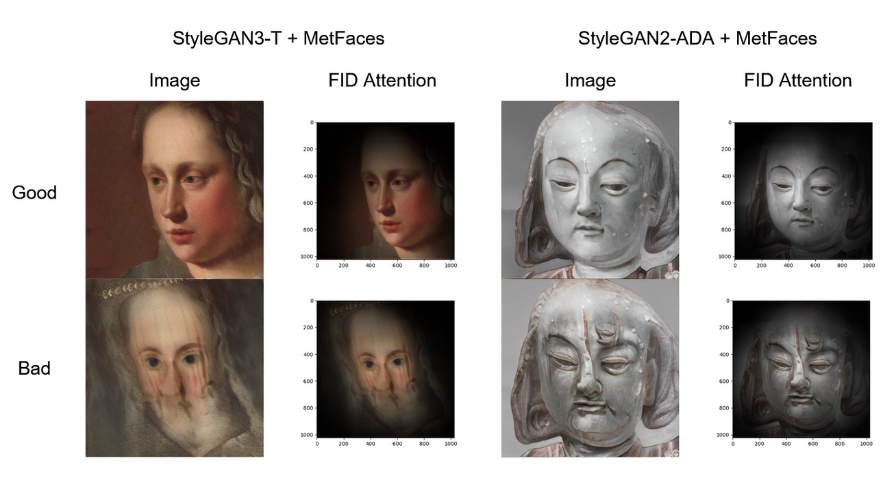
Human understanding of face images is primarily based on semantic meanings of fixed local areas, for example, ear, nose, eyes, face shape, et cetera. In our experiments, we found that FID calculations tend to focus on complex textures and shapes rather than selecting patches with semantic meaning. For example, it focuses significantly more on accessories worn, hairstyle, beard, background, anonymous occlusions, et cetera than facial features. See Figure 5 for an illustration of this behavior. Across the board, FID calculation focuses on small patches with strong patterns or textures rather than on the human face. For example, in the two good images in the first row, FID focuses almost exclusively on hair and background.
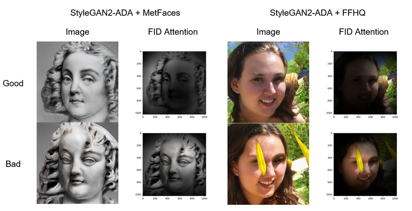
[*Figure 5. Images with their FID attention from StyleGAN2-ADA with MetFaces and FFHQ. First row good images are those picked as improved from the second row bad images. *]
However, FID does not always fail in the previously mentioned regard. In Figure 6, we demonstrate that FID can focus on the human face well, even across some good bad sample pairs. We can only consistently find this behavior in models trained with the MetFaces dataset and found that it is ubiquitous to have a blank or pure color background in images like this. We hypothesize that in this case, even if it seems FID is focusing well on the face, it is because it has nothing else to focus on. On the other hand, with FFHQ trained networks, this situation is rare. We underline that the attention areas tend to change rapidly between local feature patches and background patterns, likely due to the significant variation in background present in the FFHQ dataset.
[*Figure 6. Images with their FID attention from StyleGAN3-T and StyleGAN2-ADA with MetFaces. First row good images are those picked as improved from the second row bad images. *]
Some of these images have attention omnipresent across the entire image. In images of this category, we found that they typically have textures all over the face. Often, these textures have no correlation to the human face in human understanding. Figure 7 presents examples that fall into this category. Notice that we can only find images of this type in those labeled as “bad.” We believe this is since well-behaving images do not typically have dense textures all over the face/image.
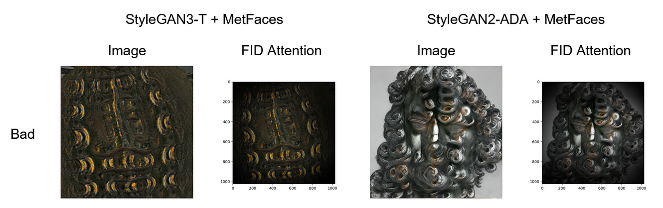
[Figure 7. Images with their FID attention from StyleGAN3-T and StyleGAN2-ADA with MetFaces. Only bad images are presented here. See the discussion in the paragraph above.]
Finally, we review the phenomenon discovered in Table 2 and detailed in Section 3.2. To be more specific, previously, we found that there exist cases where replacing bad images with better ones causes FID to improve. In this category, we found that FID calculation generally does not focus on improvements in the image’s human face structure. Instead, some new texture, pattern, or shape usually dominates the FID’s attention, causing a decrease in FID. Figure 8 illustrates this behavior. In both experiments, replacement caused FID improvement. However, in the example on the left, FID focuses almost purely on the hair and chin shape, entirely omitting the face, contrary to a human understanding of improvement. On the right, FID’s attention is performing similarly, focusing on the kerchief rather than facial features.
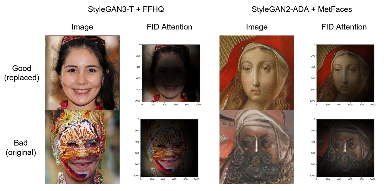
[Figure 8. Images with their FID attention from StyleGAN3-T + FFHQ and StyleGAN2-ADA with MetFaces. The top row contains the good replaced images, while the bottom contains the original bad images being replaced. In either case, replacing bad with good caused an improvement in FID. However, we hypothesize that this improvement is not due solely to the enhancement in image quality. See discussion on the paragraph above.]
5 Conclusion and Future Work
In this work, we performed a detailed analysis of FID’s focus by comparing its attention to variants of the same image. Our findings show that FID is not a good enough metric to summarize everything well in just one number. We acknowledge that designing such a general metric is challenging because of the wide range of topics and models it has to cover. However, there certainly are improvements that we can make in niche categories. In our case, we are concerned with generative modeling of human faces. Our results have shown that the generator sometimes fails catastrophically, producing images with unfathomable textures and even sometimes completely without a face, but the FID evaluation metric may not be precise enough to capture two distribution distances using Inception-V3 with these failures. To address this, we can further evaluate the quality of generated images with known face detection algorithms such as Dlib [23] and VGG-Face [22]. Since these face detection libraries are automatic and are generally very reliable, we can evaluate millions of generated samples to acquire precise estimates on the percentage of images without a visible human face. This new metric can be augmented with FID when choosing the best model during the training stage.
References
[1] I. J. Goodfellow et al., “Generative Adversarial Networks,” presented at the NeurIPS 2014, Jun. 2014. Accessed: Jun. 09, 2022. [Online]. Available: http://arxiv.org/abs/1406.2661
[2] T. Karras, T. Aila, S. Laine, and J. Lehtinen, “Progressive Growing of GANs for Improved Quality, Stability, and Variation,” presented at the ICLR 2018, Feb. 2018. Accessed: Jun. 09, 2022. [Online]. Available: http://arxiv.org/abs/1710.10196
[3] T. Karras, S. Laine, and T. Aila, “A Style-Based Generator Architecture for Generative Adversarial Networks,” presented at the CVPR 2019, Mar. 2019. Accessed: Jun. 09, 2022. [Online]. Available: http://arxiv.org/abs/1812.04948
[4] T. Karras, M. Aittala, J. Hellsten, S. Laine, J. Lehtinen, and T. Aila, “Training Generative Adversarial Networks with Limited Data,” presented at the NeurIPS 2020, Oct. 2020. Accessed: Jun. 09, 2022. [Online]. Available: http://arxiv.org/abs/2006.06676
[5] T. Karras, S. Laine, M. Aittala, J. Hellsten, J. Lehtinen, and T. Aila, “Analyzing and Improving the Image Quality of StyleGAN,” presented at the CVPR 2020, Mar. 2020. Accessed: Jun. 09, 2022. [Online]. Available: http://arxiv.org/abs/1912.04958
[6] T. Karras et al., “Alias-Free Generative Adversarial Networks,” presented at the NeurIPS 2021, Oct. 2021. Accessed: Jun. 09, 2022. [Online]. Available: http://arxiv.org/abs/2106.12423
[7] T. Salimans, I. Goodfellow, W. Zaremba, V. Cheung, A. Radford, and X. Chen, “Improved Techniques for Training GANs,” presented at the NIPS 2016, Jun. 2016. Accessed: Jun. 09, 2022. [Online]. Available: http://arxiv.org/abs/1606.03498
[8] M. Heusel, H. Ramsauer, T. Unterthiner, B. Nessler, and S. Hochreiter, “GANs Trained by a Two Time-Scale Update Rule Converge to a Local Nash Equilibrium,” presented at the NIPS 2017, Jan. 2018. Accessed: Jun. 09, 2022. [Online]. Available: http://arxiv.org/abs/1706.08500
[9] M. S. M. Sajjadi, O. Bachem, M. Lucic, O. Bousquet, and S. Gelly, “Assessing Generative Models via Precision and Recall,” presented at the NeurIPS 2018, Oct. 2018. Accessed: Jun. 09, 2022. [Online]. Available: http://arxiv.org/abs/1806.00035
[10] J. Deng, W. Dong, R. Socher, L.-J. Li, K. Li, and L. Fei-Fei, “ImageNet: A large-scale hierarchical image database,” in 2009 IEEE Conference on Computer Vision and Pattern Recognition, Jun. 2009, pp. 248–255. doi: 10.1109/CVPR.2009.5206848.
[11] R. Geirhos, P. Rubisch, C. Michaelis, M. Bethge, F. A. Wichmann, and W. Brendel, “ImageNet-trained CNNs are biased towards texture; increasing shape bias improves accuracy and robustness,” presented at the ICLR 2019, Jan. 2019. Accessed: Jun. 09, 2022. [Online]. Available: http://arxiv.org/abs/1811.12231
[12] A. Borji, “Pros and Cons of GAN Evaluation Measures: New Developments.” arXiv, Oct. 02, 2021. Accessed: Jun. 09, 2022. [Online]. Available: http://arxiv.org/abs/2103.09396
[13] S. Zhou, M. L. Gordon, R. Krishna, A. Narcomey, L. Fei-Fei, and M. S. Bernstein, “HYPE: A Benchmark for Human eYe Perceptual Evaluation of Generative Models,” arXiv, arXiv:1904.01121, Oct. 2019. doi: 10.48550/arXiv.1904.01121.
[14] E. Denton, S. Chintala, A. Szlam, and R. Fergus, “Deep Generative Image Models using a Laplacian Pyramid of Adversarial Networks,” arXiv, arXiv:1506.05751, Jun. 2015. doi: 10.48550/arXiv.1506.05751.
[15] R. R. Selvaraju, M. Cogswell, A. Das, R. Vedantam, D. Parikh, and D. Batra, “Grad-CAM: Visual Explanations from Deep Networks via Gradient-Based Localization,” in 2017 IEEE International Conference on Computer Vision (ICCV), Oct. 2017, pp. 618–626. doi: 10.1109/ICCV.2017.74.
[16] T. Kynkäänniemi, T. Karras, M. Aittala, T. Aila, and J. Lehtinen, “The Role of ImageNet Classes in Fr\’echet Inception Distance.” arXiv, Mar. 11, 2022. Accessed: Jun. 09, 2022. [Online]. Available: http://arxiv.org/abs/2203.06026
[17] K. Panetta et al., “A Comprehensive Database for Benchmarking Imaging Systems,” IEEE Trans. Pattern Anal. Mach. Intell., vol. 42, no. 3, pp. 509–520, Mar. 2020, doi: 10.1109/TPAMI.2018.2884458.
[18] Z. Liu, P. Luo, X. Wang, and X. Tang, “Deep Learning Face Attributes in the Wild,” arXiv, arXiv:1411.7766, Sep. 2015. doi: 10.48550/arXiv.1411.7766.
[19] A. Borji, “Pros and Cons of GAN Evaluation Measures.” arXiv, Oct. 23, 2018. Accessed: Jun. 10, 2022. [Online]. Available: http://arxiv.org/abs/1802.03446
[20] C. Szegedy et al., “Going Deeper with Convolutions.” arXiv, Sep. 16, 2014. Accessed: Jun. 10, 2022. [Online]. Available: http://arxiv.org/abs/1409.4842
[21] V. Kazemi and J. Sullivan, “One millisecond face alignment with an ensemble of regression trees,” in 2014 IEEE Conference on Computer Vision and Pattern Recognition, Columbus, OH, Jun. 2014, pp. 1867–1874. doi: 10.1109/CVPR.2014.241.
[22] Q. Cao, L. Shen, W. Xie, O. M. Parkhi, and A. Zisserman, “VGGFace2: A dataset for recognising faces across pose and age,” Oct. 2017, doi: 10.48550/arXiv.1710.08092.
[23] D. E. King, “Dlib-ml: A Machine Learning Toolkit,” J. Mach. Learn. Res., vol. 10, pp. 1755–1758, Dec. 2009.