Self-Learning cars under Simulator and Experiment
This report uses the Evolutionary Algorithms with a deep learning neuro network to teach a car to drive itself in the simulation. There will be a 2D planar Lidar in the simulation to detect the crash on the track. The final goal is to let the car know how to drive itself.
- Introduction
- Background about Evolutionary Algorithms
- Simulaiton preparation
- Milestones
- Progress Update (Sunday, Apr 24, 2022)
Introduction
This report uses the Evolutionary Algorithms with a deep learning neuro network to teach a car to drive itself in the simulation. There will be a 2D planar Lidar in the simulation to detect the crash on the track. The final goal is to let the car know how to drive itself.
Background about Evolutionary Algorithms
The evolution to the weights of ANNs The evolution of the connection weights draws into a self-adapting and global method for training;especially used in the reinforcement learning and recurrent network learning which based on gradient when encounter great problems. One aspect of using EAs in ANNs is to learn the weights of ANNs, that is to say to replace some traditional learning algorithms to overcome their defects. The traditional net- work weight training generally uses gradient descent method (Hertz and Krogh 1991); these algorithms are easy to fall into local optimum but can not reach the global optimum (Sutton 1986). Training the weights by certain EA can find the weight set which approaches global optimum while do not need to compute the gradient information; the individual fitness can be defined by the error between the expected output and actual output and the network complexity. The steps to use GA to evaluate the ANNs’ connection weights are as follows: Step 1 Randomly generate a group of distribution, using a coding scheme to code the weights of the group. Step 2 Compute the error function of the generated neural network, so as to determine its fitness function value. The error is larger, the fitness is smaller. Step 3 Select several individuals with the l Evolutionary algorithms are a class of stochastic search and optimization techniques obtained by natural selection and genetics. They are population-based algorithms by simulating the natural evolution of biological systems. Individuals in a population compete and exchange information with one another. There are three basic genetic operations: selection, crossover, and mutation. The procedure of a typical EA is displayed as follows: Step 1 Set t = 0. Step 2 Randomize the initial population P(t). Step 3 Evaluate the fitness of each individual of P(t). Step 4 Select individuals as parents from P(t+1) based on the fitness. Step 5 Apply search operators (crossover and mutation) to parents, and generate P(t+1). Step 6 Set t = t + 1. Step 7 Repeat step 3 to step 6 until the termination criterion is satisfied. EAs are stochastic processes performing searches over a complex and multimode space. They are population-based algorithms by simulating the natural evolution of biological systems (other population-based algorithms such as particle swarm optimization, immune algorithm, ant colony algorithm). They all have the following advantages: 1. Evolutionary algorithms can solve difficult problems reliable and fast. Thus, they are suitable for evaluation functions that are large, complex, noncontinuous, nondifferentiable, and multimodal. 2. It is a general-purpose approach that can be directly interfaced to existing simulations and models. Evolutionary algorithms are extendable and easy to hybridize. 3. Evolutionary algorithms are directed stochastic global search. They can reach the near optimum or the global maximum invariably. 4. EAs possess inherent parallelism by evaluating multipoint simultaneously. Evolutionary algorithms mainly include Evolutionary Strategy (ES), Evolutionary Programming (EP) and Genetic Algorithm (GA). The three evolutionary algorithms are consistent on the goal of using biological evolution mechanism to improve the ability of using computers to solve problems. However, they are different on the concrete measure: ES emphasizes the behavior change on the individual level, EP emphasizes the behavior change on the population level. The optimization of ANNs based on Evolutionary algorithms Neural Network has its own limitations. It is easy to fall into local minimum and sometimes hard to adjust the architecture. EAs may not be satisfactory when used in simple problems, and its performance may not be equal with the special algorithms for certain problem. But GA is robust, nonlinear and parallel, it can be commonly used for it is based on the knowledge of any special problem. EC can be used to process various problems, such as the training of the connection weights, designing the architecture, learning rules, selecting the input features, initializing the connection weights and extracting rules from ANNs. To describe neural network architecture, the main parameters are: the number of layers, the number of neurons of each layer, the connecting way between neurons, etc. Designing network architecture is to determine the combination of the parameters that is suited to solve certain problem according to some performance evaluation rules. Kolmogorov theorem speaks that three-layer feedforward network can approach any continuous function with reasonable architecture and proper weights, but the theorem has not give the way to determine the reasonable architecture, researchers can design the architecture only by the experiences. Sometimes it is difficult to construct the network artificially, what ANNs need is efficient and automatic methods to design, luckily, GA supplies a good way. Now we will discuss the recent research developments on the ANN based on EC from the three aspects: optimizing weights, optimizing network architecture and optimizing learning rules. The evolution to the weights of ANNs The evolution of the connection weights draws into a self-adapting and global method for training;especially used in the reinforcement learning and recurrent network learning which based on gradient when encounter great problems. One aspect of using EAs in ANNs is to learn the weights of ANNs, that is to say to replace some traditional learning algorithms to overcome their defects. The traditional network weight training generally uses gradient descent method (Hertz and Krogh 1991); these algorithms are easy to fall into local optimum but can not reach the global optimum (Sutton 1986). Training the weights by certain EA can find the weight set which approaches global optimum while do not need to compute the gradient information; the individual fitness can be defined by the error between the expected output and actual output and the network complexity. The steps to use GA to evaluate the ANNs’ connection weights are as follows: Step 1 Randomly generate a group of distribution, using a coding scheme to code the weights of the group. Step 2 Compute the error function of the generated neural network, so as to determine its fitness function value. The error is larger, the fitness is smaller. Step 3 Select several individuals with the largest fitness and to reserve to the next generation. Step 4 Deal with the current population using crossover, mutation and other operators and generate a new generation. Step 5 Repeat Step 2 to Step 4, make the initial weights evolve continuously, until the training goal is achieved. The main problems involved: 1. Encoding scheme (determine the expression of the connection weights of the ANN) There are two ways to encode the connection weights and the threshold values for the ANNs. One is binary encoding, the other is real encoding. Binary encoding (Whitley et al. 1990) is that each weight is expressed by fixed length 0-1 string. When the encoding length is limited, the expression precision of binary encoding is not enough; if certain precision limit is satisfied, the search space will increase correspondingly and effect the speed of the evolutionary process. Real encoding is to express each weight with a real number (Ren and San 2007); it overcomes the demerit of binary encoding, but needs to re-design the operators. Train the network Because GA is good at searching large-scale, complex, non-differentiable and multimodal spaces; it doesn’t need the gradient information of the error function. On the other hand, it doesn’t need to consider whether the error function is differentiable, so some punishments may be added into the error function, so as to improve the network commonality, reduce the complexity of the network. The results of GA and BP algorithm are both sensitive to the parameters, the result of BP algorithm also depends on the original state of the network, but BP algorithm appears to be more effective when used in local search, while GA is good at global search. On the fact of this, connection weight evolution algorithm can be implemented in the following way. First, use GA to optimize the initial weight distribution and locate some better search spaces in the solution space. Then use BP algorithm to search the optimal solution in these small solution spaces. Generally, the efficiency of the hybrid training is superior to the training methods that only use BP evolution or only use BP training (Meng et al. 2000). The problem that should be considered when using EAs to train ANNs is the permutation of the algorithm (Yao et al. 1997), that is, the algorithm converges to locally optimal solution. This is mainly because the phenomenon of several to one mapping from gene space to actual solution space. Generally speaking, it is often because of the appearance of the networks which have the same functions but different gene sequences. The permutation phenomenon caused by this reason result in the inefficiency of crossover operation; and good filial generation individuals can not be generated. Consequently EP and ES which are mainly rely on mutation operations will better restrain the detrimental effects caused by permutation than GA which is mainly depend on crossover operation. The evolution to the architecture of ANNs The network architecture is usually predefined and fixed. The design of the optimal architecture can be treated as a search problem in architecture space, where each point represents an architecture. The architecture of the ANNs has important influence on the information process ability of the ANNs, which includes the network connections and the transfer functions. A good architecture can solve problems in a satisfactory way, and doesn’t allow the existence of redundant nodes and connections. For a given problem, the process ability of an ANN with few connections and hidden neurons is limited, but if the connections and hidden neurons are too many, the noise may be trained together and the generalization ability of the network will be poor. Formerly people often used try and error method to design the architecture, but the effect overly depends on the subjective experience. With the development of EAs, people regard the design of the network as a search problem, using learning accuracy, generalization ability, and noise immunity as evaluation criterion, find the best architecture with best performance in the architecture space. The evolution of the architecture makes the ANNs can fit the network topology in different tasks. The development of architecture evolution is mainly reflected in the architecture coding and operator design. The steps of using GA to evolve the ANN architecture are as follows: Step 1 Randomly generate N architecture,and code each architecture. Step 2 Train the architecture in the individual set using many different initial weights. Step 3 Determine the fitness of each individual according to the trained result and other strategies. Step 4 Select several individuals whose fitness is the largest, directly passing on to the next generation. Step 5 Do crossover and mutation to the current population, to generate the next generation. Step 6 Repeat Step 2 to Step 5, until some individuals in the current population meet the demand. The GA selects the initial weights and changes the number of neurons in the hidden layer through the application of five specific genetic operators, that is, mutation, multipoint crossover, addition, elimination and substitution of hidden units. Addition operator and elimination operator are used to adaptively adjust the number of the neurons in hidden layers, and the addition operator is used for adding new neurons when necessary, while the elimination operator is used for preventing the network growing too much. The fitness is determined by the hidden layer size and the classification ability. The BP is used to train these weights. This makes a clean division between global search and local search. In the process of the evolution of the network architecture, the computation of the fitness often uses the randomly generated weights; this will draw into noises inevitably. In order to reduce the noises as much as possible, many researchers proposed to evolve the architecture and the weights at the same time. Yao and Liu used EP algorithm to develop a neural network automatic design system—EPNet (Yao et al. 1997). EPNet used five mutation operators: hybrid training, node deletion, connection deletion, connection addition, and node addition. Behaviors between parents and their offspring are linked by various mutations, such as partial training and node splitting. The evolved neural network prefers the node/connection deletion operations to the node/connection addition operations so as to keep the network simple. The hybrid training operator that consists of a modified BP with adaptive learning rates and the simulated annealing is used for modifying the connection weights. After the evolution, the best evolved neural network will be further trained using the modified BP. Peter. et al. thought the prospect of using GA to evolve the architecture of ANNs was limited (Peter et al. 1994). Because GA may exclude some hidden and useful networks, and the crossover operation will bring a series of problems. Compared with GA, EP uses mutation as the only gene recombination operation, it uses more natural expression to the tasks and it is more suitable for evolving the neural network architecture. The evolution to the learning rules of ANNs Different activation functions have different properties and different learning rules have different performance. For example, the activation functions can be evolved by selecting among some popular nonlinear functions such as the Heaviside, sigmoidal, and Gaussian functions (Alvarez 2002). The learning rate and the momentum factor of the BP algorithm can be evolved (Kim et al. 1996), and learning rules can also be evolved to generate new learning rules. EAs are also used to select proper input variables for neural networks from a raw data space of a large dimension, that is, to evolve input features (Guo 1992). In the traditional ANNs training, learning rules are previously assigned, such as the generalized δ rule of BP network; the design of the algorithms mainly depends on special network architecture, and it is difficult to design a learning rule when there is not enough prior knowledge of the network architecture. So we can use GA to design the learning rules of ANNs, the steps are as follows: Step 1 Randomly generate N individuals; each individual represents a learning rule. Step 2 Construct a training set, each element in it represents a neural network whose architecture and connection weights are randomly assigned or previously determined, then train the elements in the training set using each learning rule respectively. Step 3 Compute the fitness of each learning rule, then select according to the fitness. Step 4 Generate next generation by doing genetic operations to each individual. Step 5 Repeat Step 2 to Step 4, until the goal is reached. There are many parameters in learning rules. These parameters are used to adjust the network behavior, such as the learning rate can speed up the network training. At the stage of encoding, encode the learning parameters and the architecture together, then evolve the architecture, at the same time the learning parameters are evolved. The objects of evolving the learning rules are the learning rule itself and the weight adjustment rule; evolving the learning rules makes the evolved network suitable to the dynamic environment much better. Learning rules are the heart of ANNs training algorithms. Evolving the learning rules implies two basic assumptions: first, the update of weights only depends on the local information of the neurons; second, all of the connections use the same learning rule. EAs can be used to train all kinds of neural networks, irrespective of the network topology. To date, EAs are mainly used for training feed-forward neural networks, such as multilayer perceptron (Yao 1999), radial basis function network (Harpham et al. 2004), etc. Some researchers used it in recurrent neural network. With the development of EAs, many new EAs are used for evolving the ANNs, such as multi-objective evolutionary algorithm (Yen 2006), parallel genetic algorithm (Castillo et al. 2008), etc. Multi-objective evolutionary algorithm is used to evolve a set of near-optimal neural networks from the perspective of Pareto optimality to the designers, so that they can have more flexibility for the final decision-making based on certain preferences. Genetic algorithm, as a kind of heuristic method, can be utilized in many non-optimization methods. Some work utilized genetic algorithms in finding a more reasonable model architecture [7]. In order to find a desired latent space in a more efficient way, CG-GAN [5] uses a genetic algorithm to identify style transferring spaces for two images.
Simulaiton preparation
We have the F1-Tech simulator installed in the Ubuntu 18.04. The simulator is based on the ROS system. A car has five front-facing sensors that measure the distance to obstacles in a particular direction. Readings from these sensors feed into the car’s neural network. Each sensor points in a different direction, covering a frontal range of about 90 degrees. The maximum range of the sensor is 10 units. The neural network output then determines the car’s current engine and steering force. The Neural Network used is a standard, fully connected, feedforward Neural Network. It comprises 4 layers: an input layer with 5 neurons, two hidden layers with 4 and 3 neurons respectively and an output layer with 2 neurons. The weights of the Neural Network are trained using an Evolutionary Algorithm known as the Genetic Algorithm. A figure showing the simulation is listed in Figure 1.
At first there are N randomly initialised cars spawned. The best cars are then selected to be recombined with each other, creating new “offspring” cars. These offspring cars then form a new population of N cars and are also slightly mutated to inject more diversity into the population. The newly created population of cars then tries to navigate the course again and the process of evaluation, selection, recombination and mutation starts again. One complete cycle from the evaluation of one population to the evaluation of the next is called a generation.
The result is ideal. We spent some time on the training and the car can drive itself. A figure is shown in the figure 2.

Milestones
- Week 4 - 5: Select the topic and start to install the ROS and simulator.
- Week 6 - 7: Implement and tune search on the Evolutionary Algorithms.
- Week 8: Build the track in the simulator.
- Week 9: Build the nero network and start the testing.
- Week 10: Final presentation.
- Week 11: Real car experiment & Final report.
Progress Update (Sunday, Apr 24, 2022)
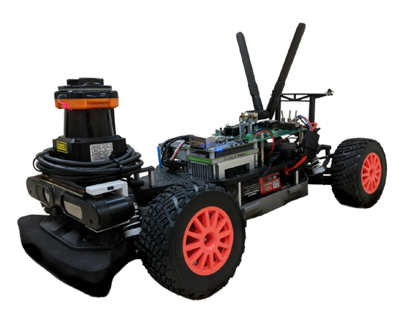
OThe Simulator for the F1-tenth is actually designed for the 1/10 scale physical vehicle to test the algorithms. The physical car model is shown in Fig.3. We transplant the simulation result to the physical car and test the result. However, the result is not ideal, even after we finish the debugging process. The reason here is the delay between the controller and the 2D planar Lidar. The timeline currently can’t match, so the crash happens. More time will be needed to finish the transplantation process. Then I can compare the traditional control VS the self learning althogrim. I will email you the result during the summer when I can finish it.
