Module 9: Explainable ML - Topic: Class Activation Mapping and its Variants
While neural networks demonstrate impressive performance across tasks, they make predictions in a black-box way that is hard for humans to understand. To alleviate the issue, researchers have proposed several ways of interpreting the behaviors of neural networks. In this survey, we focus on class activation mapping and its variants, which are popular model interpretation techniques and allow us to visualize the decision process of neural networks and ease up debugging.
- An Overview of CAM
- Class Activation Mapping
- Gradient-based CAM Variants
- Gradient-free CAM Variants
- Conclusions
- References
An Overview of CAM
Class activation mapping (CAM) and its variants (e.g. [1-8]) are techniques originally designed to obtain the discriminative image regions of a convolutional neural network (CNN) when the model is predicting a specific class during image classification, highlighting the importance of image regions that are relevant to a given class. The visualization enables us to gain insights into why neural networks are generating their outputs, whether their decision process is intuitive and if they are using spurious input-output correlations.
Since the first CAM paper [1] was introduced, there are a lot of follw-up works in this direction [2-8] and have been widely applied in models of various fields, including both CNN and vision transformer-based [9] image classification, visual question answering, and image captioning models. In this survey, we will first introduce the original CAM paper, then briefly cover four representative CAM variants categorized into two groups (i.e. gradient-based and gradient-free methods) and compare the similarities and differences between them.
Class Activation Mapping
The CAM paper [1] is specifically designed for convolutional networks with an global average pooling layer before outputs. In this section, we will first introduce GAP and then illustrate the details of CAM.
Background: Global Average Pooling
Convolutional neural networks usually consists of a sequence of convolutional layers at the beginning and one or a few fully-connected layers at the end. The fully-connected layers can take most of the parameters of the whole network and make the model prone to over-fitting. In order to solve the issue, Lin et al. [10] propose a novel architecture called Network in Network, one of the main contributions of which is to use a global average pooling (GAP) layer before outputs instead of the fully-connected layers. The GAP layer can significantly reduce the total number of the model parameters and make the model more efficienct and less prone to over-fitting.
The idea of GAP is quite simple: for a given image, if we denote the activation of channel $k$ in the last convolutional layer at spatial location $(x, y)$ as $f_k(x, y)$, then the output of the GAP layer for channel $k$ is simply $F^k = \sum_{x, y} f_k(x, y)$. Essentially, we average all the activations in channel $k$ and convert them into a single value. After we obtain the $k$-dimensional vector output from GAP, we perform a weighted sum of each element in the vector for a given class $c$, denoted as $S_c = \sum_k w_k^c F_k$, where $w_k^c$ is a parameter that is learned during training. The resulting scores are then fed into a softmax layer to generate the final output probability $Y_c=\frac{\exp(S_c)}{\sum_{c_i} \exp(S_{c_i})}$.
From GAP to CAM
CAM treats the weight terms in GAP as the importance score of $F_k$ for a given class $c$. Therefore, if we plug the expression of $F_k=\sum_{x,y} f_k(x, y)$ into the class score $S_c$, we can obtain the following equation: \(S_c = \sum_kw_k^c \sum_{x, y} f_k(x, y) = \sum_{x, y}\sum_k w_k^cf_k(x, y).\)
From the above equation, we can see that each spatial location (x, y) contributes independently to the class score. Therefore, the authors of CAM [1] define $M_c$ as their class activation map for class $c$, where the value of the spatial element $(x, y)$ is computed by: \(M_c(x, y) = \sum_k w_k^cf_k(x, y),\) where $M_c(x, y)$ directly measure the importance of spatial location $(x, y)$ for the output score of class $c$.
After we obtain the class activation map, we can perform unsampling to the size of the input image, so that we can visualize which image regions contribute the most to the prediction of class $c$.
The authors demonstrate the effectiveness of CAM, enalbing us to visualize the convolutional neural networks as well as directly adapting image classification models for object localization. While promising, one notable drawback of CAM is that they can only be applied to GAP-based convolutional networks, while a lot of the existing models have fully-connected layers at the end. In the paper, the authors show that replacing the fully-connect layers with GAP will not hurt the model performance significantly, but there indeed exists an accurary-interpretability trade-off.
Inspired by CAM, there are a number of follow-ups in this direction and we will then describe how they inherent the general idea and improve the algorithm. We will introduce four representative works and we categorize them into two groups, including gradient-based and gradient-free methods.
Gradient-based CAM Variants
In this section, we will cover two variants of CAM that uses the gradient information to obtain the class activation maps, including Grad-CAM [2] and Grad-CAM++ [3].
Grad-CAM
Grad-CAM is one of the most popular network interpretation methods in the field. Grad-CAM is a generalization of CAM and can be applied to off-the-shelf neural networks of many kinds without the need to re-train them, which is much more flexible than the original CAM algorithm.
Recall that for CAM, each element in the final class discriminative saliency map is obtained by $M_c(x, y) = \sum_k w_k^cf_k(x, y)$. Grad-CAM takes the exact formulation while changing the way of computing the weights for all the channels. Different from CAM, Grad-CAM first performs a back-propagation on the input image given a specific class $c$. Once we obtain the gradients of all the elements in the $k$-th channel, we can accumulate these gradients and treat the result as the importance score of the $k$-th channel for class $c$: \(w_k^c = \frac{1}{Z} \sum_{x, y} \frac{\partial Y_c}{\partial f_k(x, y)},\) where $Z$ is a normalization term.
After we obtain these channel weights, we can perform a weighted sum of the channel output activations and obtain the class activation maps as in CAM: \(M_c(x, y) = \sum_k w_k^cf_k(x, y).\)
We can see that the main difference between CAM and Grad-CAM is that the weights are learned during training for CAM, whereas they are computed during inference for Grad-CAM.In fact, the authors prove that when applying Grad-CAM to GAP-based convolutional neural networks, the channel weights for CAM and Grad-CAM are the same. In other words, Grad-CAM is a strict generalization of CAM.
The authors also demonstrate that Grad-CAM can be applied to a wide range of models, including image classification, visual question answering, and image captioning models. In addition, it has been recently shown that Grad-CAM can also be applied to vision transformer-based models [9]. These results demonstrate that Grad-CAM is generally applicable and much more flexible than CAM.
Grad-CAM++
Grad-CAM has two main limitations: firstly, Grad-CAM fails to localize objects in an image if the image contains multiple occurrences of the same class. In addition, Grad-CAM heatmaps often fail to capture the entire object in completeness which is important to recognition task for single object images. Therefore, Grad-CAM++ [3] was proposed to address these shortcomings.
In particular, different feature maps may be activated with differing spatial footprints, and the feature maps with lesser footprints fade away in the final saliency map. To solve this problem, GradCAM++ works by taking a weighted average of the pixel-wise gradients to calculate weights: \(w_k^c=\sum_{x,y} \alpha_{xy}^{kc} \text{ReLU}(\frac{\partial Y_c}{\partial f_k(x,y)})\).
The $\alpha_{xy}^{kc}$ terms are weighting co-efficients for the pixel-wise gradients for class $c$ and convolutional feature map $A^k$. By taking \(\alpha_{xy}^{kc} = \frac{1}{\sum_{l,m} \frac{\partial Y_c}{\partial f_k(l, m)}}\) if $\frac{\partial Y_c}{\partial f_k(x, y)} = 1$ and $0$ otherwise, all the spatially relevant regions of the input images are equally highlighted. As a result, Grad-CAM++ provides more general visualization for multiple occurrences of a class in an image and poor object localizations. In addition, the authors further show that Grad-CAM++ can be extended to tasks such as image captioning and video understanding.
Gradient-free CAM Variants
While utilizing the gradients to obtain channel weights can be helpful, researchers have shown that gradients can sometimes saturate, in which cases the above gradient-based methods can fail to generate reliable saliency maps. Thus, researchers have also proposed several gradient-free methods and we will cover Ablation-CAM [4] and Score-CAM [5] in this section.
Ablation-CAM
The authors of Ablation-CAM first present qualitative examples that when the model is very confident about its predictions, the gradients will saturate and because Grad-CAM uses the gradient information, it can generate unreliable class activation maps in these cases. To solve this issue, they propose to do ablations on each of the channels and obtain their channel weights accordingly.
Specifically, we first perform a forward pass on the neural network given an image input and get the output score $S_c$ for a given class $c$. Afterwards, we can ablate each of the channels, meaning that we manually set all the output activation values in the $k$-th channels to $0$, and the output score will be changed from $S_c$ to $S_c^k$. Intuitively, the difference between the original output score and the ablated score quantifies the importance of the $k$-th channel for class $c$, and thus we can treat this value as the channel weights in CAM: \(w_k^c = \frac{S_c-S_c^k}{S_c},\) where $S_c$ in the denominator serves as a normalization term.
Then, similar to CAM and its other variants, we can obtain the final saliency map with the computed channel weights according to the equation $M_c(x, y) = \sum_k w_k^cf_k(x, y).$
The authors demonstrate that their algorithm can outperform Grad-CAM and Grad-CAM++ both quantitatively and qualitatively. However, it should be noted that they have to perform $N+1$ times of forward passes for a single input, where $N$ is the number of channels, which requires significantly more computations than previous methods and makes them hard to use in practice.
Score-CAM
Wang et al. [5] also argue that the gradients may not be an optimal solution to generalize CAM, and thus propose a new visual explanation method named Score-CAM. This method uses global contribution of the corresponding input features instead of gradient information to encode the importance of activation maps. The first limitation of the gradient-based methods is that the gradient for a neural network may be noisy and tend to vanish due to saturation problem. Besides, there exists false confidence in gradient-based method. For example, when compared to a zero baseline, activation maps with larger weights demonstrate a lesser contribution to the network’s output in Grad-CAM. Instead of using the gradient information coming into the final convolutional layer to describe the value of each activation map, Score-CAM defines a concept called \textit{increase of confidence} and use it to express the relevance of each activation map. Specifically, given an input $X$ and a baseline input $X_b$ (e.g. an input with zero values), the contribution of the activation $A_l^k$ at the $k$-th channel of the $i$-th layer towards the model output $Y$ is defined as: \(C(A_l^k) = f(X \circ H_l^k) - f(X_b),\) where $f$ is the function represented by the neural network, $\circ$ is the Hadamard product, and $H_l^k = s(Up(A_l^k)).$$ which means that $H_l^k$ is calculated by first upsampling $A_l^k$ and then mapping each element in the input matrix into $[0, 1]$. As shown in the following figure, the pipeline is as follows: the network first extracts the activation maps and upsamples each activation maps into input size in phase 1. Each activation map is then added to the input image and then the forward-passing score of the target class is obtained. In phase 2, this process is repeated for $N$ times, where $N$ is the number of activation maps. Finally, the resulting outputs are produced by linearly combining the score-based weights and activation maps.
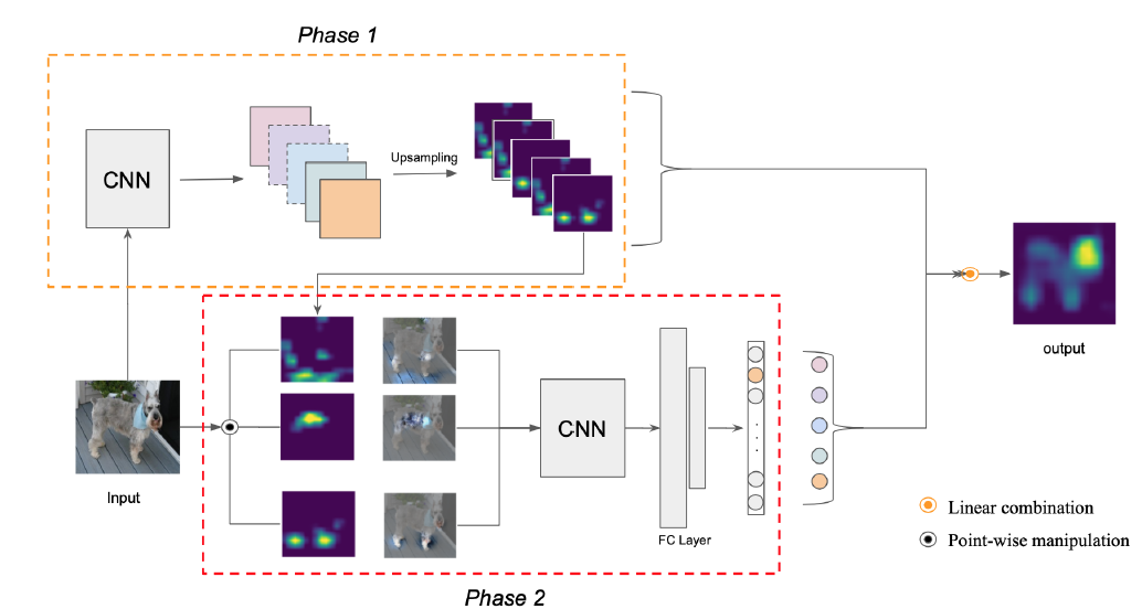
*Fig 1. Pipeline of the proposed Score-CAM.
The authors quantitively evaluate the fairness of generated saliency maps of Score-CAM on recognition tasks and its localization performance. Furthermore, the authors show that Score-CAM can be used for applications as debugging tools.
Conclusions
In summary, we introduce five ways of generating class activation maps, including both gradient-based and gradient-free methods. They all share the same idea of obtaining the saliency maps by first computing the importance scores of channels and then performing a weighted sum of channel outputs. The original CAM paper is inspiring and demonstrates promising performance, but it can only be applied to a limited class of neural networks. Grad-CAM fixes this drawback via utilizing the gradient information and has demonstrated applications in various fields. Follow-up works further refines the idea by using high-order gradients or channel-wise ablations, which may further improve the model performance in certain cases while being more computational.
References
[1] Zhou, Bolei, Aditya Khosla, Agata Lapedriza, Aude Oliva, and Antonio Torralba. “Learning deep features for discriminative localization.” In Proceedings of the IEEE conference on computer vision and pattern recognition, 2016.
[2] Selvaraju, Ramprasaath R., Michael Cogswell, Abhishek Das, Ramakrishna Vedantam, Devi Parikh, and Dhruv Batra. “Grad-CAM: Visual explanations from deep networks via gradient-based localization.” In Proceedings of the IEEE international conference on computer vision, 2017.
[3] Chattopadhay, Aditya, Anirban Sarkar, Prantik Howlader, and Vineeth N. Balasubramanian. “Grad-CAM++: Generalized gradient-based visual explanations for deep convolutional networks.” In Proceedings of the IEEE winter conference on applications of computer vision, 2018.
[4] Ramaswamy, Harish Guruprasad. “Ablation-CAM: Visual explanations for deep convolutional network via gradient-free localization.” In Proceedings of the IEEE winter conference on applications of computer vision, 2020.
[5] Wang, Haofan, Zifan Wang, Mengnan Du, Fan Yang, Zijian Zhang, Sirui Ding, Piotr Mardziel, and Xia Hu. “Score-CAM: Score-weighted visual explanations for convolutional neural networks.” In Proceedings of the IEEE conference on computer vision and pattern recognition workshops, 2020.
[6] Muhammad, Mohammed Bany, and Mohammed Yeasin. “Eigen-CAM: Class activation map using principal components.” In Proceedings of the international joint conference on neural networks, 2020.
[7] Belharbi, Soufiane, Aydin Sarraf, Marco Pedersoli, Ismail Ben Ayed, Luke McCaffrey, and Eric Granger. “F-CAM: Full resolution class activation maps via guided parametric upscaling.” In Proceedings of the IEEE winter conference on applications of computer vision, 2022.
[8] Hsia, Hsuan-An, Che-Hsien Lin, Bo-Han Kung, Jhao-Ting Chen, Daniel Stanley Tan, Jun-Cheng Chen, and Kai-Lung Hua. “CLIPCAM: A Simple Baseline For Zero-Shot Text-Guided Object And Action Localization.” In Proceedings of the IEEE international conference on acoustics, speech and signal processing, 2022.
[9] Dosovitskiy, Alexey, Lucas Beyer, Alexander Kolesnikov, Dirk Weissenborn, Xiaohua Zhai, Thomas Unterthiner, Mostafa Dehghani et al. “An image is worth 16x16 words: Transformers for image recognition at ccale.” In Proceedings of the international conference on learning representations. 2020.
[10] Lin, Min, Qiang Chen, and Shuicheng Yan. “Network in network.” In Proceedings of the international conference on learning representations, 2014.